A 2-dimensional geometry for biological time
Progress in Biophysics and Molecular Biology
We frame several features of biological time with a 2-d manifold to accommodate autonomous biological rhythms both for individuals and comparisons.
Abstract
This paper proposes an abstract mathematical frame for describing some features of biological time. The key point is that usual physical (linear) representation of time is insufficient, in our view, for the understanding key phenomena of life, such as rhythms, both physical (circadian, seasonal …) and properly biological (heart beating, respiration, metabolic …). In particular, the role of biological rhythms do not seem to have any counterpart in mathematical formalization of physical clocks, which are based on frequencies along the usual (possibly thermodynamical, thus oriented) time. We then suggest a functional representation of biological time by a 2-dimensional manifold as a mathematical frame for accommodating autonomous biological rhythms. The “visual” representation of rhythms so obtained, in particular heart beatings, will provide, by a few examples, hints towards possible applications of our approach to the understanding of interspecific differences or intraspecific pathologies. The 3- dimensional embedding space, needed for purely mathematical reasons, allows to introduce a suitable extra-dimension for “representation time”, with a cognitive significance.
Keywords: Biological rhythms, Allometry, Biological rhythms, Circadian rhythms, Heartbeats, Rate variability
A 2-dimensional Geometry for Biological Time
Abstract
This paper proposes an abstract mathematical frame for describing some features of biological time. The key point is that usual physical (linear) representation of time is insufficient, in our view, for understanding key phenomena of life, such as rhythms, both physical (circadian, seasonal …) and properly biological (heart beating, respiration, metabolic …). In particular, the role of biological rhythms do not seem to have any counterpart in mathematical formalization of physical clocks, which are based on frequencies along the usual (possibly thermodynamical, thus oriented) time. We then suggest a functional representation of biological time by a 2-dimensional manifold as a mathematical frame for accommodating autonomous biological rhythms. The “visual” representation of rhythms so obtained, in particular heart beatings, will provide, by a few examples, hints towards possible applications of our approach to the understanding of interspecific differences or intraspecific pathologies. The 3-dimensional embedding space, needed for purely mathematical reasons, allows to introduce a suitable extra-dimension for “representation time”, with a cognitive significance.
Keywords: biological rhythms, allometry, circadian rhythms, heartbeats, rate variability.
1 Introduction
Living phenomena displays rather characteristic and specific traits; among these, manifestations of temporality and of its role are particularly remarkable: development, variegated biological rhythms, metabolic evolution, aging, …. This is why we believe that any attempt at conceptualizing life phenomena — be it only partially — cannot avoid addressing such temporal aspects that are specific to it. In that which follows, we will examine this question from different angles in view of providing a first attempt at synthesis.
The intuitive “geometry of time” in physics was (and often still is) based, first, on the absolute Newtonian straight time line. This was later enriched by the order structure of Cantor type real numbers, an ordered set of points, topologically complete (dense and without gaps). Thermodynamics and the theories of irreversible dynamics (phase transitions, bifurcations, passing into chaos, …) have imposed an “arrow” upon classical time, by adding an orientation to the topological and metric structure. But it is with relativity and quantum physics that the theorization of time has led to rather audacious reflections. In the first case, to give only one example from a very rich debate which goes so far as to introduce a circular time (proposed by Gödel as a possible solution to Einstein’s equations) to Minkowski space: by means of its famous causality cone, this space explains, within the framework of a unified geometry of space-time, the structure of any possible correlation between physical objects, in special relativity.
In quantum physics the situation is maybe even more complex or, in any event, less stable. We go from essentially classical frameworks to a sometimes two-dimensional time (in accordance with the structure of the field of complex numbers with regard to which Hilbert spaces are defined, the theoretical loci of quantum description), up to the audacity of Feynman’s temporal “zigzags” Feynman & Gleick 1967. This latter approach is a very interesting example of intelligibility by means of a “geometric” restructuring of time: the creation of antimatter would cause within the symmetry (charge, parity, time) a symmetry breaking in terms of charge, while leaving parity unchanged. Global symmetry is then achieved by locally inverting the arrow of time. Another approach, with similar motivations, is that of the fractal geometry of space-time, specific to the “scale relativity” proposed by Nottale 1993: in it, time is reorganized upon a “broken” line (a fractal), which is continuous but non-derivable. Further interesting reflections, along similar lines, may be found in Le Méhauté, Nigmatullin & Nivanen 1998.
Physics however will remain but a methodological reference for our work, because the analysis of the physical singularity of living phenomena Bailly & Longo 2006, 2011 requires a significant enrichment of the conceptual and mathematical spaces by which we make inert matter intelligible. One of the new features which we introduce consists in the usage that we will make of the “compactification” of a temporal straight line: in short, we will try to mathematically understand rhythms and biological cycles by means of the addition of “fibers” (a precise mathematical notion, introduced summarily below) which are orthogonal to a physical time that remains a one-dimensional straight line. From our standpoint, a living being is a true “organizer” of time; by its autonomy and action, it confers it a more complex structure than the algebraic order of real numbers, but also more than any organization one could propose for the time of inert matter. In short, the time of a living organism, by its specific rhythms, intimately articulates itself with that of physics all the while preserving its autonomy. We would therefore like to contribute to making the morphological complexity of biological time intelligible, by presenting a possible geometry of its structure, as a two dimensional manifold.
The first paragraph will introduce the theme of biological rhythms. One consequence of our approach is the possibility of mathematically giving what we hope to be more precise and relevant meaning to notions that are usually treated in a rather informal fashion and unrelated between one another, such as those of representation time, physical time vs. biological rhythms, … and this within a rigorous mathematical frame.
1.1 Methodological remarks
Let’s recall that physics, in its history, was constituted according to major dimensional constants (gravitation, the speed of light, Plank’s constant — with dimensions, respectively: acceleration, speed, action). What is striking, in biology, is the presence of a few major invariants with no dimension, those that are specified in the rhythms of which we will speak below. The mathematization of physics concentrated on invariants, among which the above constants, but also those of “objective determinations”, which we address in length in Bailly & Longo 2006, 2011. We suggest here to start with these rare invariants, these constants and rhythms which are to be found in biology, because, beyond the physico-chemical, the structural stability of living phenomena is not “invariant”, physically speaking: it is profoundly imbued with variability.
Observe also that in physics, time is mostly described as a parameter of the state functions describing a system. The phenomena encountered in biology, however, seem to trigger the need of other theoretical strategies and this at many different temporal levels of organization (physiology, ontogenesis, phylogenesis, …). We will provide a geometrical scheme of biological time that stresses the crucial role of time in life and allow to understand some of the above features mainly through the use of two theoretical concepts.
The first one, which we will discuss in depth latter, is the ubiquity of rhythms in biological temporal organization. There is indeed few features that are ubiquitous in biology but the iteration of similar processes seems to be one of them. We will however make a clear distinction between two type of cyclicity encountered in living systems.
The second concept is a way to understand the constitution and maintenance of biological organization, both in phylogenesis and embryogenesis, that we formalized by the notion of anti-entropy in Bailly & Longo 2009. That approach allows the addition of a new theoretical aspect of time irreversibility in biological systems, that completes and adds up to the thermodynamical irreversibility driven by the notion of entropy. At the level both of evolution and embryogenesis, this irreversibility manifests itself by the increase of complexity of the organism (number of cells, number of cell types, cell networks — neural typically, geometrical complexity of the organs, constitution of interacting yet differentiated levels of organization, …).
Methodologically, by a duality with physics, in Bailly & Longo 2009 time is understood as an operator (like energy in Quantum Physics), not as a parameter. This makes time a fundamental observable of biology (like energy in physics) and it gives meaning to its key role in “biological organization”, since rhythms organize life.
2 An abstract schema for biological temporality.
2.1 Premise: Rhythms
We will introduce a second dimension of time, associated to the endogenous internal rhythms of organisms, a dimension of time which we will represent as compacified ( topology[1]).
We denote this compacified time as , which we can represent as a sort of “circle” with a “radius” (where is the proper biological time): this circle expresses the temporal circularity, the iterative component, that is specific to internal rhythms.
2.2 External and internal rhythms
We will distinguish two types of rhythms associated with biological organization, each referring to a distinct temporal dimension (below, we will note them as and , respectively):
- (Ext)
- “external” rhythms, directed by phenomena that are exterior to the organism, with a physical or physico-chemical origin and which physically impose themselves upon the organism. So these rhythms are the same for many species, independently of their size. They express themselves in terms of physical, hence dimensional, periods or frequencies (s, Hz) and the invariants are dimensional; they are described with regard to the dimension of physical time (in ). Examples: seasonal rhythms, the 24 hours-cycle and all their harmonics and sub-harmonics, the rhythms of chemical reactions which oscillate at a given temperature, etc.
- (Int)
- “internal” rhythms, of an endogenous origin, specific to physiological functions of the organism, depend on purely biological functional specifications. These rhythms are characterized by periods which scale as the power of the organism’s mass and, when related to the life span of the organism which scales in the same way, they are expressed as pure numbers (they have no physical dimensionality). Invariants are therefore numeric. We propose to describe them with regard to a new compacified “temporal” dimension , with a non-null radius, the numeric values then corresponding to a “number of turns”, independently of the effective physical temporal extension (we have mentioned some examples: heartbeats, breathings, cerebral frequencies, etc.).
We will now, even if we must be somewhat repetitive, describe further how these rhythms take place in biological organization, which is precisely what we would like to provide account for:
-
The external rhythms (Ext) are to be identified with physical time (typically measured by a clock) determined universally — their temporal features does not depend of the biological system we consider. Key examples include
circadian, circannual or tidal cycles. The effects or the relevancy of these cycles depend of course on the organism that we consider (with possible sexual dimorphism). For example, diurnal and nocturnal animals are in phase
opposition, whereas tides are mainly relevant for marine organisms, and especially in the foreshore. Whatever organism we consider, the period and the phase of these rhythms are the same as they are dependent on external physical
events. In order to be a little more precise, this rhythms are generally associated with a double process: the physical process, outside the living system (and which can be very precisely predicted) and its “shadow” inside the
system which is kept synchronized by so-called “Zeitgeber” (light for circadian cycle for example). This distinction leads in particular to a specific inertia, encountered for example in the “jet lags” phenomenon.
Simple chemical oscillations inside an organism will fall in this category too, since their period is determined by physical principles, however their phase depends on a specific organism (a specific trajectory) since it is the organism which constructs this chemical system.
As a result, this kind of rhythms, and their subharmonics, can be considered in the usual physical way and represented by terms like .
-
The second kind of rhythms, the endogenous biological cycles in (Int), do not depend directly on external physical rhythms. They could be called autonomous or eigen rhythms and scale with the size of the organism (frequencies
brought to a power
of the mass, periods brought to a power
), which is not the case with constraining external rhythms which impose themselves upon all (circadian
rhythms, for example). Such rhythms are encountered when we consider the heart rate, the respiratory rate, the mean life span, …, see Savage et al. 2004 or Lindstedt & Calder III 1981 for example. This rhythms are naturally associated with the
number of their iterations (they can be seen as dual variables), and these numbers provide a natural way of speaking of the age of a biological system, yet different of the time measured by a clock. The distinction between
replicative and chronological aging for yeasts, is a clear example of this situation, see Fabrizio et al. 2004.
It is worth noting that this kind of rhythms leads to the use and the study of pure numbers instead of quantities with a physical dimensionality (such as intervals of physical time). Moreover these numbers seem, at least in certain cases, to have invariant[2] properties, a clear and impressive example of this is the mean number of heartbeat (or respiration) during life which is almost invariant among mammals.
In summary, endogenous biological rhythms:
- are determined by pure numbers (number of breathings or heart beats over a lifetime, for example) and not, in general, by dimensional magnitudes as is the case in physics (seconds, Hertz, …);
- depend on the adult mass of the organism that we consider, by following the allometric law (for heterotherms, the temperature is involved too);
- in our approach, they are analyzed and put into relation to each other by adding an additional compacified “temporal” dimension (an angle, actually, like in a clock), in contrast to the usual physical dimension of time, a line, non-compacified and endowed with dimensionality.
Since these endogenous rhythms co-exist with physical time, we consider a temporality of a topological dimension equal to formed by the direct product of the non-compacified part, the real straight line of the variable (the physical time parameter) and, as a fiber upon the latter, the compacified part, a circle , of which the variable is . Since we consider a two-dimensional time, with a second dimension associated with specific biological invariants, our approach is very different of the usual approach of biological time in terms of dynamical systems, which allows to tackle different kind of questions, like synchronization or stability (see for example the noteworthy book of Winfree 2001), but do not deal with these invariants.
The idea of using supplementary compacified dimensions in theoretical physics has been introduced by Kaluza and Klein Overduin & Wesson 1997, and is still widely used in unification theories (string, superstring, M-theory, …). There are of course major differences between these uses of compacified dimensions and ours. First they concern mostly the addition of space-dimensions; second these dimensions are not observable in physics, whereas they are clearly observable in biology. In our approach, the projection of this second dimension on physical time leads to quantities that have the dimension of a time; their mean follows the allometric law, as such they are parametrized by a mass (or, equivalently, by an energy; here one may see again the dual role of energy vs. time as parameter vs. operator, the duality w. r. to Quantum Physics we mentioned and extensively used in Bailly & Longo 2009).
We insist that the endogenous rhythmicities and cyclicities are not physical temporal rhythms or cycles as such, as they are iterations of which the total number is set independently from the empirical (temporally physical) life span. As we said, they are pure numbers, a few rare constants (invariants) in biology. Our aim is that of a geometric organization of biological time which, by the generativity specific to mathematical structures, would also enable us to derive meaning and to mathematically correlate diverse notions. The text itself constitutes the commentary and the specification of the following schemata, which are meant to “visualize” the two-dimensionality which we propose for the time specific to living phenomena.
3 Mathematical description
We first consider both external and internal rhythms; later, we will mainly focus on internal rhythms of organisms (we can take as a paradigmatic example the heart rate of mammals). We begin by providing a qualitative draft of our scheme to show its geometrical structure in figure 1, then we will quantify its parameters and explain more precisely their meaning.
3.1 Qualitative drawings of our schemata
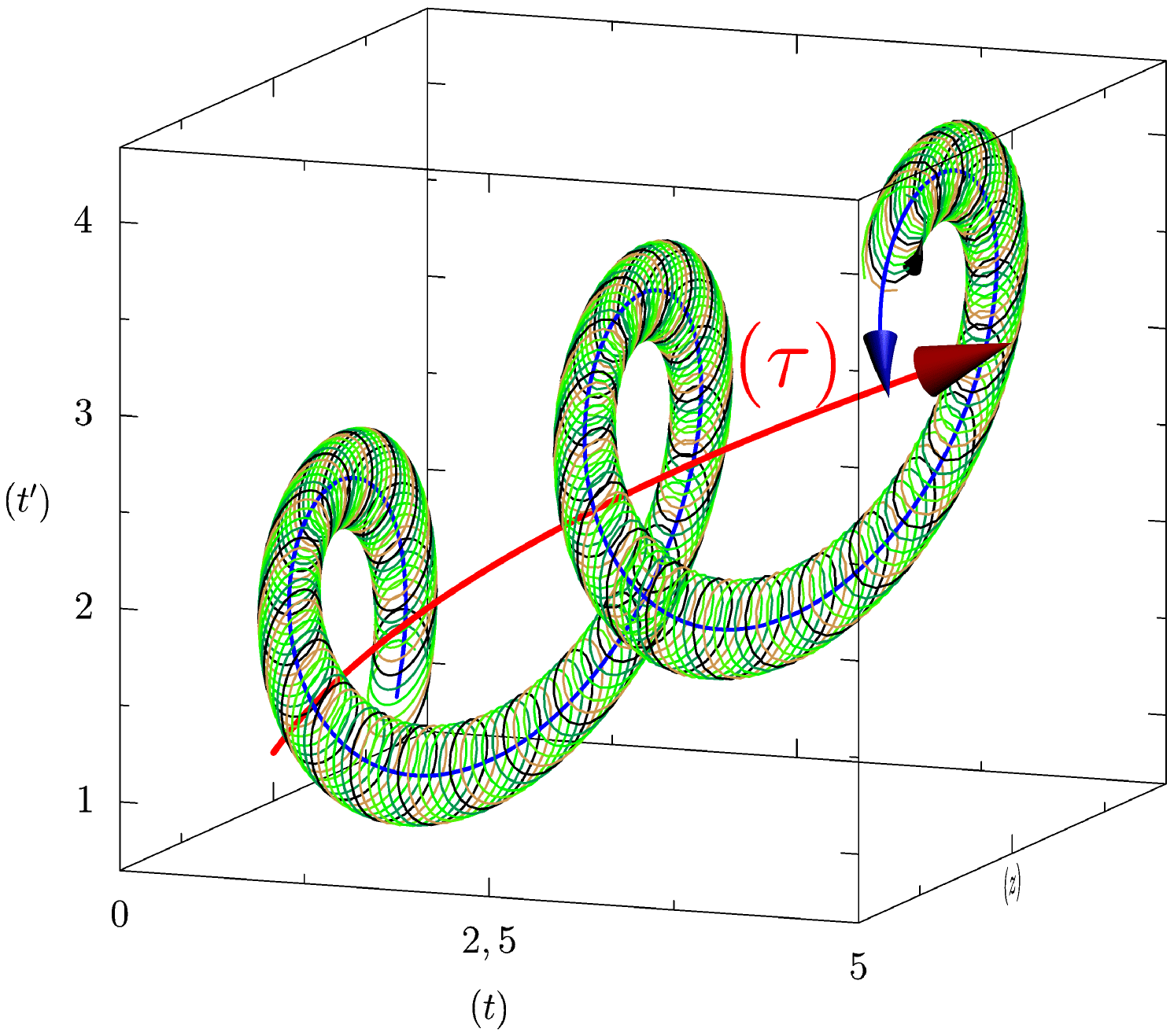
Following the aforementioned ideas, biological time is a (curved) surface: thus, it will be described in 3-dimensions (the embedding space). Note that, if we were considering only biological rhythms, our 2-dimensional manifold would be a cylinder: the (oriented) line of physical time times the extra compacified dimension. The situation is more complicated, in view of the further, physical rhythms we want to take into account. They do not require an extra dimension, but they “bend” the cylinder, by imposing global (external) rhythms. Thus, a proper biological rhythm is represented by what we may call a “second order helix”, that is, a helix that is obtained (is winding) over a cylinder, , which, in turn, is winding around a bigger cylinder, , of which the axis is the line . As basic reference, we choose orthogonal Cartesian coordinates. Physical time, which is oriented by thermodynamic principles of irreversibility and is measured by a clock as in classical or relativistic physic, will be the first axis of our reference system and will enable the characterization of instants and the measurement of durations. The second axis, , will be associated with the proper irreversibility of biological time (for example the irreversibility of embryogenesis or, just, of “living”, see 5). As such, it will represent the biological age, or the internal irreversible clock of the organism we consider. The and axis are oriented in the usual way ( towards the right and pointing upwards). The third axis, , (see 1) is generated by the mathematical need of a 3-dimensional embedding space; yet, we claim that it has a biological meaning that will become clear later, in section 3.2.
We consider the surface of the cylinder as parametrized by (the physical time) and (the compacified time).
Let’s then take a further step by gradually making explicit the functional dependencies.
-
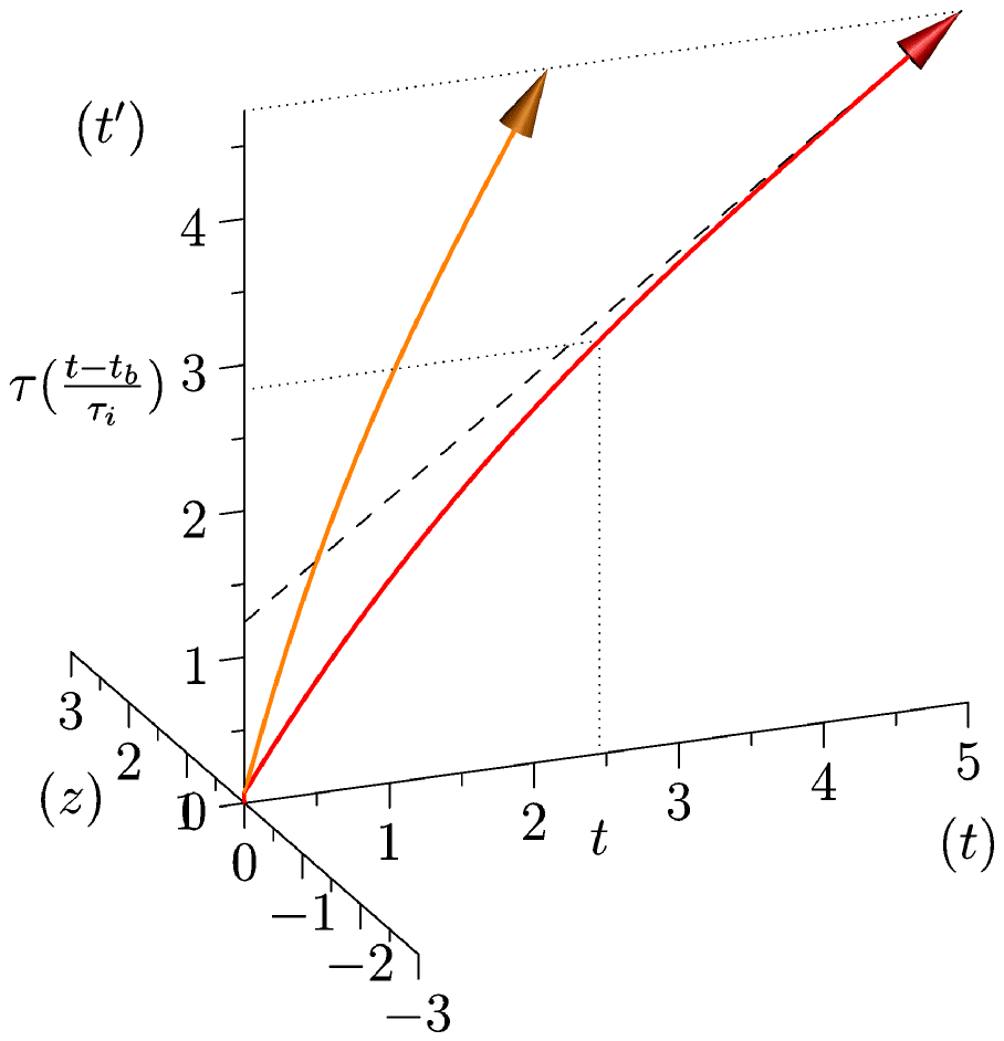
The average progression with respect to
will be represented by a function
.
is a growing function due to the irreversibility of biological time, and has a decreasing derivative due to the decrease of activity during
development and aging.
is the physical time of a biological event of reference (time of fecundation for example).
is a characteristic time of the biological activity of the adult: for example, the mean “beat to beat” interval under standardized conditions (other reference systems can be chosen such as the mean time taken to attain 98% of adult
mass, life expectancy, respiratory interval, …). This value represents, as a function of physical time, the age of the system inasmuch this age is biologically relevant (see figure
2a: the graph of
lies on the
plane). Set then:
(1) -
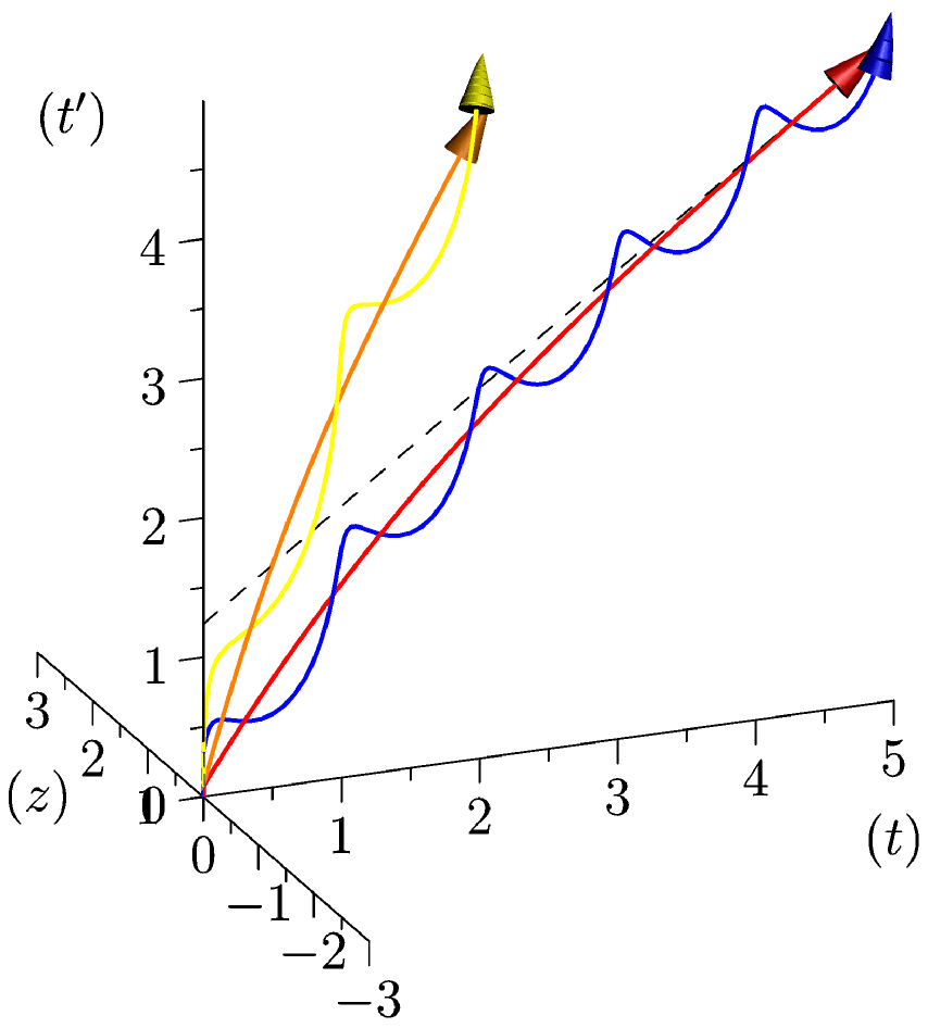
We next consider a physical (external) rhythm of period
(its pulsation is then
) that affects the activity rate of the organism — the circadian rhythm, for example, leads to
hours. This produces a winding spiral or helix,
(see figure 2b: here we need the third dimension
for the embedding space of our manifold). In the definition of
,
represents the impact of this physical rhythm on biological activity:
(2) The term is proportional to the number of iterations of the compacified time during one period of the physical rhythm, as such it can be considered as the temporal weight of this rhythm for an organism (mean number of heartbeat during a day, for example), it allows to understand that a year is more important for a mouse and for an elephant. As a consequence the radius of is proportional to both the impact of this rhythm on biological activity, and on the weight of this rhythm in terms of number of iteration of the endogenous rhythm considered during one period of the physical rhythm.


Figure 2: Qualitative Illustration of the first components of our model. left, the function , which represents the global age of an organism: this age increases at a greater pace during development and slows down progressively, see section 5. In orange a small mammal (a mouse for example) and in red a bigger one (an elephant). The life span of the first is shorter than one of the second. Right, in blue (and yellow), a physical rhythm has been added (this rhythm is very slow for illustrative purposes). Notice that this physical rhythm has the same period for both animals, but one of its iteration has a greater weight for the smaller animal. -
We can finally add a biological (internal) rhythm, which depends on an increasing function
(see figure 3).
has a proper biological meaning: for example, if we impose
, with
when the heart begins to beat[3],
is the number of heartbeats of the organism at time
, and thus the mean maximum of
, obtained when death occurs, does not depend on the organism we consider (among mammals, typically). Set then, for
as in equation 2:
(3)
3.2 Quantitative scheme of biological time
Now, one of the simplest way to define more precisely is to use and more precisely the length of the curve defined by . We obtain then for the instantaneous pulsation, where is the derivative of (thus ) and the other components are the derivative of the remaining coordinates in equation 3:
| (4) |
The term is here for (physical) dimensionality reasons: since our metric has the dimension of a frequency, and , the derivative of the first component of the vector in equation 2, has no dimension, then we need to introduce this coefficient whose dimension is a frequency[4].
When we can simplify 4 to:
| (5) |
Now, if we consider hibernating animals, or frozen organisms, we have situations where the physical time flows normally but where the biological time almost stops or even totally stops. For , even in the frozen case, biological time would flow with . It seems then natural to suggest that . Moreover, for , we go back to allometric relations, since, in this case, is proportional to . Now, is proportional to , by allometry, and, thus, , which is a frequency, to , as it should be.
Another way to express this is to say that physical time per se does not make biological organization get older: it is only when there is a biological activity (which in return is of course always associated with physical time) that aging appears.
We can now even give a meaning to the third, , axis: since is on the plane, a positive corresponds to a positive , by equation 3, and it is associated with a slowdown of biological activity (sleep, for example), whereas the negative values are associated to a faster pace (wake for example).
As a fundamental feature of the model that we will analyze next, we assume that the speed of rotation with respect to the compacified time is constant, which leads to a radius .
| (6) |
This assumption “geometrizes” time even further: acceleration and slow-down will be seen as contraction and enlargement of a cylinder in §4.4.2. In that section, as an application, we will develop a geometrical analysis of biological rate variability, and, as an example, we will consider heart rate. Note that this radius is the dimension accommodating the biological rhythms, thus it is not a physical dimension (it is a pure number). Our assumption is consistent with the idea that each iteration along the compacified time contributes equally to aging.
4 Analysis of the model
In this section we will explore the various biological aspects our approach allows to put together, mainly on the questions of interspecific and intraspecific allometry and on (heart) rate variability.
4.1 Physical periodicity of compacified time
Since provides the frequency of the biological rhythm, it is interesting to look for a simple analytical expression of the period associated. To do so, we perform a Taylor development (under the hypothesis ) of the inverse of equation 5, and as a result we obtain an approximation of the physical time associated with an iteration of the compacified time (the time between two heartbeats for example):
| (7) |
We can observe several things here. First, for adults (i.e.: and it does not depend on the size of the organism we consider) the result has the form . As a consequence, when we take different species, there is no variation of the ratio ( ) between the continuous and the period components of the biological rates. Alternatively the ratio between the rates of the biological rhythm during the slow period of the physical rhythm (sleep for example) and during the fast period (wake) does not depend of the species either. This result holds experimentally (see for example Savage et al. 2004 and Mortola & Lanthier 2004).
On the other side, the relationship between this two rates is not linear in intraspecific variations (i.e.: when is not constant, mainly during development), and the variation of the coefficient of the rhythmic component is far greater than that of the steady (continuous) component . This mathematical deduction agrees with experimental results, since Massin et al. 2000, for example, find that the continuous component varies like while the sinusoidal part (associated with the circadian rhythm) varies like for humans (between 2 months and 15 years).
4.2 Biological irreversibility


We can now look more precisely at the second axis, , of our reference system. Since this aspect of biological time is irreversible and flows in the same direction than physical time ( is an increasing function of ), in equation 2 should increase with respect to this direction. When this condition is met, we will say that these times are “cofluent”. This can be easily mathematized by looking at the partial derivative of the component of (obtained with the dot product by the unitary vector ) with respect to :
| (8) |
We obtain then three different scenari, assuming that tends to be a constant for adults (and seniors), written . We then use equation 5 to derive their observable consequences:
- .
- In this case, biological age and the physical clock are cofluent, and the minimum rate is achieved during adult sleep (figure 3a and 3d).
- .
- In this case, they are minimally cofluent, the derivative tends to zero (during night or winter) when the organism grows older, that is the rate of the biological rhythm tends to during the (physical) time of little biological activity. It seems to be particularly relevant for hibernation (figure 3b and 3e)….
- .
- in this case they are no longer cofluent, the nullification of the biological rate would appear during development, and, as a result, the slowest biological rhythm would appear during sleep of young individuals (figure 3c and 3f).
This case analysis has an actual correspondence with empirical data for the first two cases (see for example Hellbrugge et al. 1964; Cranford 1983). We believe that theoretically biological time should be always cofluent so that the third case should never be realized. Indeed, the existing data, which are mostly given for humans, confirm that case does not hold (young individuals have slow rhythms, during sleep typically, which are faster than adults slow rhythms).
It would be nice that our theoretical deduction, excluding, like in physical reasoning, the third mathematical possibility as meaningless, were empirically confirmed in large phyla. Conversely it would be also interesting if this theoretical derivation leads to the discovery of species where also the third case is realized.
4.3 Allometry and physical rhythms
When we consider organisms with different adult masses ( ), we obtain a variation of according to the scaling relationships ( ), whereas does not change. As a result, this change corresponds to a dilatation of the axis (as far as is concerned) whereas the physical rhythm modifies the geometry of biological time because the variations it triggers are anchored to the physical value (see figures 2a, without physical rhythm, and 2b, with physical rhythms.).
Then, it is the interplay between physical rhythms and biological ones that breaks the symmetry (by dilatation) between organisms of different (adult) masses that have the same temporal invariants (most mammals for example). As a result, in this situation, the physical conditions can be seen as constraints or frictions on biological temporal organization. Our point of view can be compared to the dimensionless time in West & Brown 2005, but they only consider the autonomous aspect of biological time, thus not considering this important interplay.
An other way to illustrate these aspects is to count the lifelong number of iterations of cycles: for biological cycles, this number does not vary much when considering different species, whereas it is strictly proportional to life span for physical ones.
4.4 Rate Variability
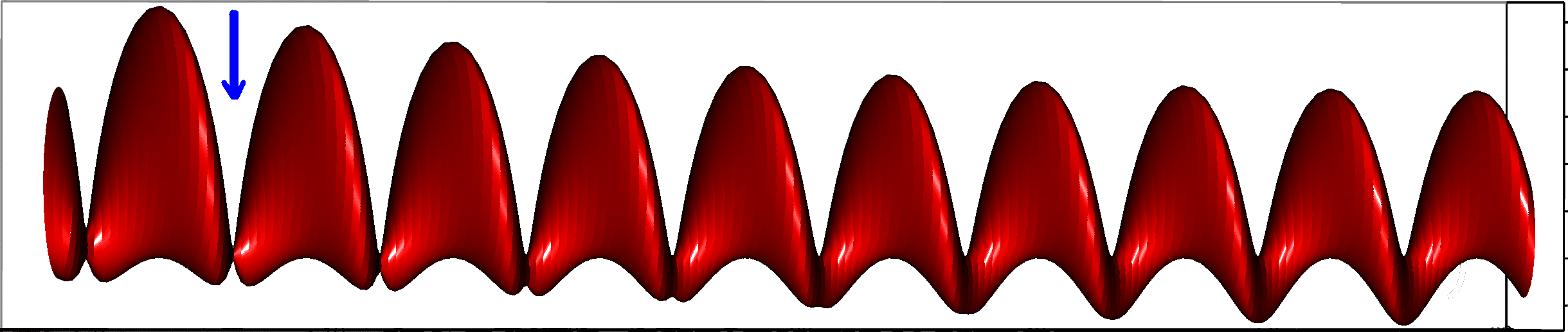
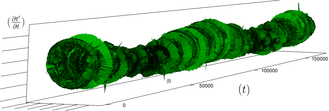
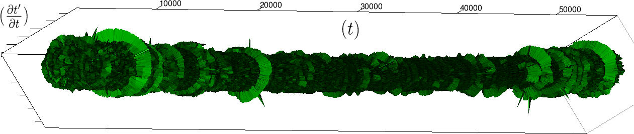
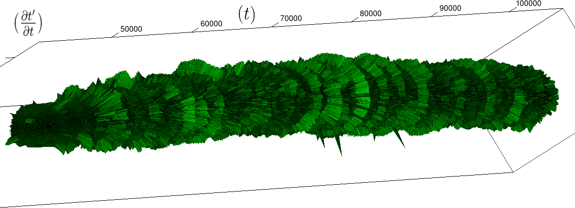
Let us first introduce informally the applications we will hint to in this section, where the data are obtained from the medical references in place. Our approach to biological time leads naturally, as we will further specify, to a representation by a cylinder whose radius is proportional to the cardiac rate. If we assume that n heartbeats yield a complete rotation around the cylinder, then a faster heart rate would appear as a circular outgrowth (a sudden increase in the radius). In this representation, a healthy individual has a complex cardiac dynamics during the day, with frequent rhythms’ accelerations of varying length (from seconds to many hours). This shows up in the figures by the many circular outgrowths of different radii. On the contrary, an individual with an artificially regulated pace (with a pacemaker, say) gives a relatively smooth cylinder. The last figure below corresponds to a sudden cardiac death, without particular symptoms.
Of course we do not provide a theoretical determination of spontaneous biological rates variability, but just a geometrical representation. As a matter of fact in our framework, it is quite straightforward to explore the structure of biological rhythms and of their variations. More precisely, we can easily and effectively represent raw datas (for example the series of “beat to beat” interval over time). As a result, we obtain more than a qualitative schema: it is a theoretical grounded representation of the “anatomy” (and pathological anatomy) of biological time. First we need to see how we can use scales in our framework.
4.4.1 Renormalization
If we want to consider iterations of the compacified time as an iteration of an other compacified time we obtain and , then by some sort of renormalization using the principle of constant speed for the compacified time, one has:
| (9) |
So . This result is exactly (modulo a global dilatation of the and axis by a factor ) what we obtain if we construct directly our system at the level of iterations.

4.4.2 Rate Variability


If we look at the function obtained by taking the derivative of with respect to , we obtain:
| (10) |
Here, instantaneous heart rate, , appears directly as the radius of compacified time, (which has the physical dimension of a frequency now).
If the experimental time of each heartbeat is given in a list , we obtain a discrete empirical version of , renormalized by :
| (11) |
where is an estimation of which may be soundly considered constant during the few days of the measure. is an estimation of . Both of these values are estimated by using equation 5 and . We obtain a 2-dimensional structure by using triangles between adjacent points, that is to say for , the triangles and . It is worth mentioning that this approach allows to obtain an empirical version of too.
The renormalization by allows to observe directly the correlations between consecutive heartbeats (a full circle) and the contrasts between a group and its neighbors (see figure 4), thus discriminating easily between the sleep situation (no correlations wider than heart beat) and the healthy wake state (correlations at each scale). The latter is indeed characterized by a succession of randomly spaced outer circle (see figure 5).
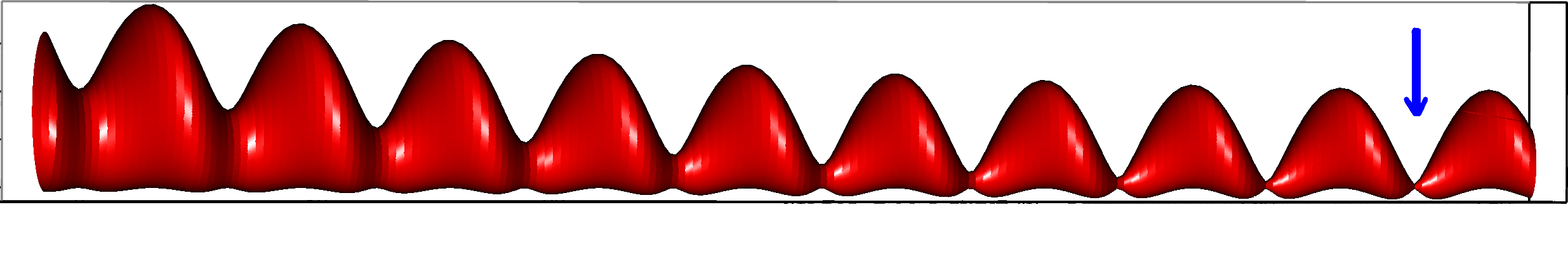
Moreover this representation may be useful to study cases of heart diseases and even aging, since this situations are characterized by an alteration of heart rate variability. We illustrate this alteration in cases of sudden cardiac death in figure 6 computed with datas from the The Sudden Cardiac Death Holter Database, see Goldberger et al. 2000. This figure evidentiate the anatomy and the pathological anatomy of heart rhythms and suggests the extension of this approach to other biological rhythms which are less explored.
- Figure 6a is an example of a healthy case, which is characterized by a complex temporality during wake.
- In figure 6b, (intermittent) pacing leads to an excessively regular cylinder, with few heart rate variability.
- Atrial fibrillation in the figure 6c (a kind of arrhythmia, see comments in figure 6) leads to an “hairy” structure, which represents a strong short term randomness (few correlations between successive heartbeats).
- Last but not least the figure 6d is not associated with a specific diagnosis (put aside sudden cardiac death at time ) but it clearly shows a very simpler structure than the healthy case.
Our approach allows to discriminate all these various cases by rather striking geometrical differences. Wavelet analysis is often used for the same purpose, but this approach is based on a massive reorganization of datas, through a decomposition in various components, whereas we only perform a geometrical and synthetic composition of them.

5 More discussion on the general schema 1.
5.1 The evolutionary axis , its angles with the horizontal and its gradients
The central line , see figure 1, is the “result” of the various components (physical time, external and internal rhythms) and it is supposed to refer to a “physiological” time associated to the evolution of the organism over the course of its life. In order to better understand the different chronological parts of life, this “axis” may be decomposed in distinct segments, each being characterized by their angle, , with regard to the abscissas (the angle under consideration then becomes that of the tangent), connected by zones with a fast curvature around specific times . We will in particular distinguish five parts (with unequal lengths).
- Around (which would correspond to the fertilization of the egg that will form the organism or to a mutation which generates a new species), a new segment begins with a very large angle ( for example) and consequently with a very high gradient. This segment will correspond to embryogenesis.
- Around , there occurs a first curvature of the axis in order to initiate a segment of which the angle (and the gradient) still remains high (at , for example). Time would correspond to birth[5] and the following segment to growth (development).
- Around , we would have a new curvature generating a medium sized angle ( for example) with a gradient approaching ; would correspond to the apparition of the reproductive faculty (age of puberty[6]) and to the entering into the phase of adult maturity.
- Around , we would have another curvature generating a small angle segment ( for example) with a weak gradient; would correspond to the period of loss of fecundity (menopause, eventual andropause)[7] and to the beginning of aging as such.
- Around the axis becomes horizontal ( , ) and is definitely broken; represents the moment of death.
Concerning the various durations (namely that of the life span - ), we know by the above mentioned laws of scaling generally encountered in biology, that these durations scale according to the organism approximately by , where is the mass of the adult organism.
If we now consider as being the “speed” of evolution of the physiological time with regard to the physical time , we would make the following remarks which motivate the various gradients of :
- between and this speed is very high: initial cell divisions, morphogenesis, setting in of the first functionalities;
- between and , the speed remains high; it corresponds to growth, to development, to the completion of the setting in of functionalities, to a high metabolism;
- between and the speed is moderate; it corresponds to the regularity of the metabolic reactions, of cellular renewal, etc., that are characteristic of adult age;
- between and , the speed is low: lowering of the metabolic rate, of cellular regeneration, of activity; this corresponds to aging;
- after the speed is null: it is the death of the organism.
5.2 The “helicoidal” cylinder of revolution : its thread , its radius
In our qualitative analysis (see 1) we have a cylinder of revolution , with a radius , which is winded as a helix having a thread of around the axis, without touching this axis but faithfully following its changes of direction.
The thread of this helicoidal cylinder can be assimilated to a period; it corresponds to the external cyclical rhythms imposed upon the organism by its environment (annual, lunar, circadian cycles, for instance, see §.2.2(EXT)), which are independent physico-chemical rhythms that we have taken into account in the first paragraph; they are essentially of a physical origin and are imposed upon all organisms exposed to them. The case will be evoked below.
5.3 The circular helix on the cylinder and its thread
This circular helix , with a thread , is winded around the surface of the cylinder (it is a “second order” helix because the winding cylinder is also helicoidal). We consider the thread of this helix (which is also a period) to refer to the compacified time (the circle which generates this cylinder) introduced here and associated to the internal biological cycles of the organism which are also independent (or almost) from the environment; this is the case, let’s recall, for example, of cardiac and respiratory rhythms, of the rhythms of biochemical cascades, etc. (see §. 2.2(Int)). Let’s also recall that the period associated to these cycles also scale by , at least from (and also practically from ).
To summarize, we thus have, from a biological standpoint, in addition to the objective physical time (evidently still present and relevant):
- a general temporality of biological evolution (the axis);
- a temporality associated to the external rhythms (the helicoidal cylinder winded around this axis from a distance) that are characterized by the thread ;
- a temporality associated to the internal rhythms involving a compactification of time: the helix with a thread at the surface of the cylinder.
We should also note that if the radius of the helicoidal cylinder becomes null, it will be reduced to a helix winded around and the internal cyclicity will tend to disappear as such (there remains only the external rhythms that are physical). If we may consider the general schema we have presented to concern mainly the properties of the animal world, this last case, where , mainly concerns plant. In this sense, the non nullity of , that is, the two-dimensionality of the cylindrical surface, should be associated to the greater autonomy — the rhythms of the central systems, typically — and to the autonomous motor capacity which the animal enjoys comparatively to vegetal organisms, the two being obviously correlated. Actually, the rhythms (metabolic, chlorophyllian, of action — activation of organs…) of plants are often completely subordinated to the physical external rhythms.
Of course, there is no clear-cut transition, no well-defined boundary between animal and plant life forms in particular in the marine flora/fauna. For this reason, we find the representation of the passing from the one to another in the form of a continuum to be adequate: the continuous contraction of the helicoidal cylinder which tends towards being a helix, which is a line (the time of plants). The non observability of the difference between animal and plant, in some “transitional” cases, would correspond to an interval of biologically possible measurement, with no phase transition (of the type of life form) that is clear or discontinuous. Once the limit, the helicoidal line, is reached, even the three-dimensional embedding space can be collapsed onto the two dimensions: the rhythm becomes the oscillation of one measurement (of chlorophyllian activity, for example) with regard to the axis of oriented physical time (the spiral is flattened into a sine, for example) as is the case in many periodic physical processes.
5.4 On the interpretation of the ordinate
Let’s return now to our questioning regarding the interpretation we can give to the ordinate . In a certain sense, it is generated by the compacified fiber of the temporal rhythms specific to living phenomena. More specifically, it is mathematically necessary as a component of the three-dimensional embedding space of helixes produced by the direct production of the physical time t and of the compacified time , which are, according to our hypothesis, two independent dimensions. We already hinted to a possible biological meaning of the coordinate. Then, what could the ordinate correspond to, from a biological standpoint?
If we define a speed for the passing of time comparatively to in a way that is similar to the definition of , we will have ; at the inverse of (we have ), this velocity is small at first but continues to grow when (or ) grows.
In the case where the organism under consideration is the human being, an interpretation promptly comes to mind. The velocity ’ would correspond to the subjective perception of the speed of the passing of the “specific” or physiological time : at first very slow, and then increasingly rapid with aging. In such case, would be the equivalent of a subjective time. One will notice that, from the quantitative standpoint, if between and (the area of the adult phase) we confer with the value of approximately, as we have already indicated above, the speed of the passing of time with regard to objective physical time ( ) coincides more or less with the subjective perception of the passing of this time ( ) (in fact, ).
As it is matter, here, of human cognitive judgment of the time flow, we are aware of its historical contingency. The remarks below, thus, are just informal preliminaries to forthcoming reflections, where the historicity of young vs. old age perception of time, for example, should be relativized to specific historical cultures and social frames. We then leave the reader to have any reflection regarding the subjective perception of time during youth and old age. We can imagine that such thoughts will coincide with ours, if we belong to the same “culture” (time which passes slowly while young and, later, very quickly…).
In what concerns organisms other than human beings, of which we do not know if they have a subjective perception of the speed of the passing of physiological time , it is more difficult to assign a clear status to this dimension of (although certain relatively evolved species seem likely to express impatience, for example, or to construct an abstract temporal representation by exerting faculties of retention and especially of protention). So would this dimension not begin to acquire a concrete reality only with the apparition and development of an evolved nervous system (central nervous system, brain)? But then what of the bacterium, the amoeba, the paramecium…?
Actually, it may be possible to somewhat objectivize the approach by advancing a plausible hypothesis regarding the general character of : we could consider that it is a question of a “temporality” that is associated to the “representational” dimension. Let’s explain.
Since living organisms are endowed with more or less capacity for retention and protention (possibly pre-conscious “expectation”), we propose (temporarily, this is ongoing work) to base ourselves on the following qualitative argument: the element of physiological time is associated to the element of physical time and to by the evident relation ; it stems from this that can be written as or as
It is then tempting to see in the first factor the minimal expression of an element of “retention” (for physiological time, relatively to physical time) and in the second the corresponding expression of an element of “protention”. The product of the two would generate the temporality component of a “representation” which borrows from the “past” and from the “future”, as constitutive of the flow of biological time. As all living organisms appear to be endowed with both a capacity for retention — as rudimentary as it may be — and with a protentional faculty (even more rudimentary maybe), the generality of the dimension would be preserved and the “representational” capacity (at least in this elementary sense) appears as being a property of living phenomena, see Longo & Montévil 2011. This property, for conscious thought, could even be extended to subjectivity in accordance, in the specific case of the human being, with the phenomenological analysis with which we began: would be a form, as elementary as infinitesimal, of the “extended present”, in the husserlian tradition, described by other analyzes, such as the coupling of oscillators in Varela 1999.
Finally, it would be the two-dimensionality — (physical time) (representation time) — which would enable to mark out the temporality of living phenomena, which may be represented in the geometrical way as we have described in this paper.
References
- Bailly, F., F. Gaill & R. Mosseri. 1993. “Orgons and biolons in theoretical biology: Phenomenological analysis and quantum analogies.” Acta Biotheoretica 41 (1–2): 3–11. doi: 10.1007/BF00712769.
- Bailly, F., & G. Longo. 2006. Mathématiques & sciences de la nature: la singularité physique du vivant. Hermann. (Cited on page 3).
- _________. 2009. “Biological organization and anti-entropy.” Journal of Biological Systems 17 (1): 63–96. doi:10.1142/S0218339009002715. (Cited on pages 3 sq., 6).
- _________. 2011. Mathematics and the natural sciences; The Physical Singularity of Life. London: Imperial College Press. (Cited on page 3).
- Bailly, F., G. Longo & M. Montévil. 2011. “A 2-dimensional geometry for biological time.” Progress in Biophysics and Molecular Biology 106 (3): 474–484. issn: 0079-6107. doi: 10.1016/j.pbiomolbio.2011.02.001.
- Bak, P., C. Tang & K. Wiesenfeld. 1988. “Self-organized criticality.” Physical review A 38 (1): 364–374. doi:10.1103/PhysRevA.38.364.
- Botzung, A., E. Denkova & L. Manning. 2008. “Experiencing past and future personal events: Functional neuroimaging evidence on the neural bases of mental time travel.” Brain and Cognition 66 (2): 202–212. doi:10.1016/j.bandc.2007.07.011.
- Bourgine, P., & J. Stewart. 2004. “Autopoiesis and cognition.” Artificial Life 10:327. doi:10.1162/1064546041255557.
- Chaline, J. 1999. Les horloges du vivant: un nouveau stade de la théorie de l’é volution? Hachette Littératures.
- Cranford, J.A. 1983. “Body temperature, heart rate and oxygen consumption of normothermic and heterothermic western jumping mice (Zapus princeps).” Comparative Biochemistry and Physiology - A 74 (3): 595. doi:10.1016/0300-9629(83)90553-4. (Cited on page 19).
- Edelman, G.M., & G. Tononi. 2000. “Reentry and the dynamic core: neural correlates of conscious experience.” In Neural Correlates of Consciousness: Empirical and Conceptual Questions, edited by T. Metzinger, 139–151. MIT Press.
- _________. 2001. A universe of consciousness: How matter becomes imagination. Basic Books.
- Fabrizio, P., S. D. Pletcher, N. Minois, J.W. Vaupel & V.D. Longo. 2004. “Chronological aging-independent replicative life span regulation by Msn2/Msn4 and Sod2 in Saccharomyces cerevisiae.” FEBS Letters 557 (1–3): 136–142. doi:10.1016/S0014-5793(03)01462-5. (Cited on page 5).
- Feynman, R.P., & J. Gleick. 1967. The character of physical law. MIT press. (Cited on page 2).
- Goldberger, A.L., L.A.N. Amaral, L. Glass, J.M. Hausdorff, P.C. Ivanov, R.G. Mark, J.E. Mietus, G.B. Moody, C.-K. Peng & H.E. Stanley. 2000. “PhysioBank, PhysioToolkit, and PhysioNet: Components of a New Research Resource for Complex Physiologic Signals.” Circulation 101, no. 23 (June): e215–e220. doi:10.1161/01.CIR.101.23.e215. (Cited on pages 25, 27, 29).
- Hellbrugge, T., J.E. Lange, J. Rutenfranz & K. Stehr. 1964. “Circadian periodicity of physiological functions in different stages of infancy and childhood.” Annals of the New York Academy of Sciences 117 (1 Photo-Neuro-Endocrine Effects in Ciradian Systems, with Particular Reference to the Eye): 361–373. doi: 10.1111/j.1749-6632.1964.tb48193.x. (Cited on page 19).
- Horsfield, K. 1977. “Morphology of branching trees related to entropy.” Respiration Physiology 29 (2): 179. doi: 10.1016/0034-5687(77)90090-1.
- Le Méhauté, A., R. Nigmatullin & L. Nivanen. 1998. Flèches du temps et gé ométrie fractales. Hermès. (Cited on page 3).
- Le Van Quyen, M. 2003. “Disentangling the dynamic core: a research program for a neurodynamics at the large-scale.” Biological Research 36:67–88. doi: 10.4067/S0716-97602003000100006.
- Lecointre, G., H. Le Guyader & D. Visset. 2001. Classification phylogéné tique du vivant. Belin.
- Lindstedt, S.L., & W.A. Calder III. 1981. “Body size, physiological time, and longevity of homeothermic animals.” Quarterly Review of Biology: 1–16. doi: 10.1086/412080. (Cited on page 5).
- Longo, G., & M. Montévil. 2011. “Protention and retention in biological systems.” Theory in Biosciences 130 (2): 107–117. issn: 1431-7613. doi: 10.1007/s12064-010-0116-6. (Cited on page 35).
- Massin, M.M., K. Maeyns, N. Withofs, F. Ravet & P. Gerard. 2000. “Circadian rhythm of heart rate and heart rate variability.” Archives of Disease in Childhood 83 (2): 179–182. doi: 10.1136/adc.83.2.179. (Cited on page 15).
- Mortola, J.P., & C. Lanthier. 2004. “Scaling the amplitudes of the circadian pattern of resting oxygen consumption, body temperature and heart rate in mammals.” Comparative Biochemistry and Physiology - A 139 (1): 83–95. doi:10.1016/j.cbpb.2004.07.007. (Cited on page 14).
- Nottale, L. 1993. Fractal space-time and microphysics: towards a theory of scale relativity. World Scientific. (Cited on page 2).
- Overduin, J.M., & P.S. Wesson. 1997. “Kaluza-Klein Gravity.” Physics Reports 283:303–380. doi:10.1016/S0370-1573(96)00046-4. (Cited on page 6).
- Peters, R.H. 1986. The ecological implications of body size. Cambridge U. P.
- Petitot, J. 2003. “The neurogeometry of pinwheels as a sub-Riemannian contact structure.” Journal of Physiology, Paris 97 (2-3): 265–309. doi: 10.1016/j.jphysparis.2003.10.010.
- Rosen, R. 1991. Life itself: a comprehensive inquiry into the nature, origin, and fabrication of life. Columbia U. P.
- Savage, V.M., J.F. Gilloly, W.H. Woodruff, G.B. West, A.P. Allen, B.J. Enquist & J.H. Brown. 2004. “The predominance of quarter-power scaling in biology.” Ecology 18:257–282. doi: 10.1111/j.0269-8463.2004.00856.x. (Cited on pages 5, 14).
- Schmidt-Nielsen, K. 1984. Scaling. Cambridge U. P.
- Szpunar, K.K., J.M. Watson & K.B. McDermott. 2007. “Neural substrates of envisioning the future.” Proceedings of the National Academy of Sciences 104 (2): 642. doi:10.1073/pnas.0610082104.
- Van Gelder, T. 1999. “Wooden iron? Husserlian phenomenology meets cognitive science.” In Naturalizing Phenomenology: Issues in Contemporary Phenomenology and Cognitive Science, edited by J. Petitot, F.J. Varela, B. Pachoud & J.M. Roy, 245–265. Stanford U. P.
- Varela, F.J. 1999. “The specious present: A neurophenomenology of time consciousness.” In Naturalizing phenomenology: Issues in contemporary phenomenology and cognitive science, edited by J. Petitot, F.J. Varela, B. Pachoud & J.M. Roy, 266–314. Stanford U. P. (Cited on page 35).
- Vaz, N.M., & F.J. Varela. 1978. “Self and non-sense: an organism-centered approach to immunology.” Medical Hypotheses 4 (3): 231–267. doi: 10.1016/0306-9877(78)90005-1.
- Waddington, G.H. 1977. “Stabilisation In Systems: Chreods and epigenetic landscapes.” Futures 9 (2): 139–146. issn: 0016-3287. doi: 10.1016/0016-3287(77)90006-4.
- West, G.B., & J.H. Brown. 2005. “The origin of allometric scaling laws in biology from genomes to ecosystems: Towards a quantitative unifying theory of biological structure and organization.” Journal of Experimental Biology 208 (9): 1575–1592. doi:10.1242/jeb.01589. (Cited on page 19).
- West, G.B., J.H. Brown & B.J. Enquist. 1997. “A General Model for the Origin of Allometric Scaling Laws in Biology.” Science 276 (5309): 122–126. doi: 10.1126/science.276.5309.122.
- _________. 1999. “The Fourth Dimension of Life: Fractal Geometry and Allometric Scaling of Organisms.” Science 284 (5420): 1677–1679. doi: 10.1126/science.284.5420.1677.
- Winfree, A.T. 2001. The geometry of biological time. Second. Springer Verlag. (Cited on page 6).