Protention and retention in biological systems
Theory in Biosciences
We suggest a simple functional representation of biological protention and introduce abstract notions of biological inertia and extended present.
Abstract
This article proposes an abstract mathematical frame for describing some features of cognitive and biological time. We focus here on the so called extended present as a result of protentional and retentional activities (memory and anticipation). Memory, as retention, is treated in some physical theories (relaxation phenomena, which will inspire our approach), while protention (or anticipation) seems outside the scope of physics. We then suggest a simple functional representation of biological protention. This allows us to introduce the abstract notion of biological inertia.
Keywords: Memory and Cognition, protention, retention, biological time
Protention and retention in biological systems
Abstract
This paper proposes an abstract mathematical frame for describing some features of cognitive and biological time. We focus here on the so called “extended present” as a result of protentional and retentional activities (memory and anticipation). Memory, as retention, is treated in some physical theories (relaxation phenomena, which will inspire our approach), while protention (or anticipation) seems outside the scope of physics. We then suggest a simple functional representation of biological protention. This allows us to introduce the abstract notion of “biological inertia”.
Keywords : Memory and Cognition ; protention ; retention ; biological time.
Introduction
The notions of “memory” and “anticipation” are analyzed here from a temporal perspective. By this, we propose a simple mathematical approach to retention and protention that are apparently shared by all organisms, albeit rudimentarily. Moreover, in life phenomena, memory is essential to learning and it is oriented towards action, the grounding of protention. Our approach will allow to address the issue of what we call “biological inertia”, a form of “continuation” of ongoing action, derived from the notions above. The frame is purely mathematical and abstract: only practitioners will be able to give values to our coefficients and develop, possibly, concrete applications of the approach, from cell biology to human cognition. Our aim is to give a precise and relevant meaning to notions that are usually treated in a rather informal fashion and unrelated between one another, such as those of time of representation, time of retention and time of protention.
A long phenomenological tradition introduces an important distinction between memory and retention, on the one hand, and anticipation and protention on the other. In short, the common meaning of “memory” seems to essentially refer to a “conscious reconstruction” of something that was experienced (very well put by Edelman as a “brain which sets itself back into a previously experienced state”). Anticipation would be its temporal opposite — the awareness of an expectation, of a possible future situation. Memory and anticipation do not, a priori, have a biological characteristic time, a notion which is essential to our analysis. In our approach, instead, possibly pre-conscious retention is to be seen as an extension of the present; it is the present which is “retained”, during a brief interval of time (related to what will be called its characteristic time) for the objective of the action (and of perception), it is a form of extension of the immediate past into the present. For example, when listening to a word or a phrase, we retain the part which has already occurred for a certain (characteristic) duration of time. The mental duration of a phrase, particularly of a musical “phrase”, is needed for grasping meaning or a melody (see for example Perfetti and Goldman 1976; Nicolas 2006): it is the present which leaves a trace the time necessary for action or, possibly, for subsequent awareness. But protention (as preconscious anticipation) is essential to appreciate a melody or understand a phrase. When reading, the analysis of saccadic eye movements demonstrates that we first look at least at half of the word following the one we are reading, see Wildman and Kling 1978. This protentional behaviour participates in the reconstruction of meaning: we appear to make sure of the meaning of the word we are reading by making a partial guess upon the following word.
Technically, protention will be given by a temporal mirror image, as it extends retention forwards into time. Protention is, above all, the tropism inherent to action performed by any life form. This point is at the center of our approach: we call retention and protention these particular aspects of memory and of anticipation that are specific to all life forms – a sort of present which is extended in both directions. Thus we do not limit our analysis to the phenomenological use of these words, inasmuch it limits their meaning to situations that can be examined through conscious activities. We believe that this extension to pre-conscious activities remains compatible with (and helps to understand) its classical usage, particularly such as described by Van Gelder 1999 and Varela 1999 who develop the concepts of intentionality, retention and of protention, introduced and discussed in length by Husserl in his analysis of human consciousness.
In this paper, it is then a question of trying to propose an elementary modelization of these inevitably fuzzy notions, one which is as rudimentary as possible, but one that can nevertheless support discussions regarding their precise conceptualization and their increasingly thorough mathematization. The introduction of the notions of “biological inertia” and “global protention” are, typically, a consequence of the generative power of mathematics.
To our aim, we will define some basic principles and more specific notions, after some methodological preliminaries.
Methodological remarks
This paper belongs to series of texts Bailly and Longo 2011, 2008, 2009; Bailly, Longo, and Montévil 2011 whose attempted aim is not to reconstruct the physico-mathematical complexity of some aspects of biology, but to propose firstly and above all a proper biological perspective. We believe that the theoretical differentiation between theories of inert and of living phenomena requires, among other things, a change in the relevant parameters and observables. As long as the actions of living organisms, including their cognitive performances which occur the moment that life appears (in this sense, we speak of protention and of retention in the amoeba or the paramecium), are analyzed within physical space-time, the physico-mathematical takes precedent over the specificity of the biological. For example, the formidable mathematics of morphogenesis, from phyllotaxy to the analysis of the fractal structures of organs, organize the results of friction in the growth of living organisms according to physical geodesics. This friction is nevertheless shaped within physical space-time (fractality optimizes the occupation of physical space, the exchange of energy by a surface within a volume …). In all of these cases, the spatio-temporal and energetic parameters and observables enable a very interesting and often technically very difficult analysis. This is an approach of the physical complexity of living phenomena and of its material structures. We could also say the same of analyses of networks of cells, of which the most complex are neural networks. Informational interaction, often a gradient of energy, enables to develop a theory, now very rich from the mathematical standpoint, of these formal networks of which increasingly important applications are being considered for the construction of machines that are somewhat intelligent (at last).
In this paper, our mathematics will not go beyond a few equations which could be presented to high school students. What matters in our view is approaching biological time according to its own specificity, by starting with some invariants which appear to be exclusively specific to living phenomena, as we did in Bailly and Longo 2011, or with properties that are not treated by current physical theories, as protention here. In Bailly, Longo, and Montévil 2011, we proposed a two dimensional representation of biological time as a mathematical frame to accomodate the autonomous (internal) biological rhythms (cardiac, respiratory, metabolic rhythms …). In the perspective of this paper, one may understand the expectation or anticipation of a rhythm to iterate, as a minimal form of protention: once rhythms are installed, the organism is “tuned” to (and “expects”) their iteration.
Before developing a further geometrization of biological-time, we will face yet another taboo of physicalism in biology: the inverted causality specific to protention. We will not present a physical theory of teleonomy, but will use as data the evidence of protentional behaviours that may be observed in any life form. When the paramecium, encircled by a ring of salt, tries after many attempts to break through the obstacle, risking its own life and possibly even succeeding Misslin 2003, we can take note of the retention/memory-learning of what we see and of the ensuing teleonomic gesture (a protention) and develop an adequate theory (see Saigusa et al. 2008). Likewise, when we hear that the brain, prior to a saccadic eye movement, in an obvious anticipation, prepares the corresponding primary cortex which is apt to receive the new signal (see Berthoz 2002), there is certainly an underlying physico-chemical mechanism which will one day enable to grasp the phenomenon by means of physical causality, a causality which may need to be invented. For the moment, let’s consider these phenomena as a form of protention to be analyzed (correlated, formalized …) by a theory specific to living phenomena, even if it has no correspondence or meaning within current physical theories. Then, the unification with the physico-chemical theories may be better considered, in order to evidentiate the physico-chemical components which underlie these phenomena. As a matter of fact, unification will be possible only when we will have two theories to compare to one another, both theories being as mathematized as possible. We are talking about unification and not reduction, since physicists aim to unify the relativistic and quantum fields and not perform a reduction of the one theory to the other: string theory and non-commutative geometry aims the construction of a new unified frame which presents a new perspective for both theories. The mathematics to be found in the following pages will give us the advantage of formalization: it forces to specify concepts and to stabilize them as much as possible (this is what mathematics is first about). Maybe that which follows is false, but it should then be possible to say so in relation to a precise formulation.
1 Characteristic time and correlation lengths
The notion of “characteristic time”, which we inherit here from physics, appears to be very important in biology as well: it concerns the unity of the living individual because, for example, fluxes and their transport entail lengths and, therefore, relevant transport times. We will also speak of characteristic times for retention and protention.
For example, according to the size of the organism, there appears to be two sorts of transport processes. For large organisms, it would be of a “propagational” type ( velocity, along networks and “channels”) with a typical correlation length of , where represents the characteristic time. For smaller organisms (cells, for example), it would rather be of a “diffusional” type (diffusion coefficient , due to molecular diffusion processes) and the typical correlation length would be .
We stress the difference regarding dependency in function of time: linear in one case, as a power of in the other.
Two complementary remarks:
- The size of the organism also affects structures determining the mode of transport, for example the respiratory function (oxygen transport): in the case of small organisms (insects, for example) the transport is performed by tracheas (or even pores), multitudes of little cylinders where the air diffuses in order to reach the cells. In the case of large organisms (fish, mammals), transportation and exchanges are performed by means of gills or of lungs, centralized anatomic structures which present the fractal geometries we evoked above and which enable to conciliate difficultly compatible constraints (efficiency, steric limitation, homogeneity), and then by various sorts of vascular systems. Transportation, in this last case, is also much more of a “propagational” type (even if diffusion does play a role, namely in bronchioles).
- These considerations essentially apply to various structural aspects responding to identical functions. The functional aspect responds for its part very generally to common scaling laws (the metabolism which corresponds particularly to oxygen intake, the variegated rhythmicities, the relaxation times …). It therefore appears that the modes of transport associated to identical functions can be different and can correspond to different anatomic structures (tracheas, gills, bronchial trees/lungs). This is the well-known phenomenon of analogy of structures in evolutionary biology.
Finally, account taken of these remarks, since the characteristic times mostly scale as , where is the mass of the intended organism (see Lindstedt and Calder III 1981; Savage et al. 2004), it is necessary to expect the correlation lengths to scale differently according to the mode of transport: respectively in and in , following the definitions of and .
In the sequel, our characteristic times will more precisely refer to “relaxation times”, still in analogy to physics (see next footnote), yet in properly biological frame, in relation to retention and protention.
1.1 Critical states and correlation length
The physics of criticality and self-organized systems has massively entered the domain of biology since early ideas by Nicolis and Prigogine 1977, Bak, Tang, and Wiesenfeld 1988, Kauffman 1993 … We further extended this approach, in direct reference to far from equilibrium systems in the sense of Prigogine, by considering living entities as being in an “extended critical situation”, beyond the pointwise analysis of critical transitions proper to physical theories, see Bailly and Longo 2008.
It is interesting now to consider that physical criticality is associated with a so-called critical slowdown (see for example Suzuki, Kaneko, and Takesue 1982: the relaxation time of a system tends to infinity when it goes near the critical point. The qualitative meaning of these situations in biology is that the effect of a stimuli would take a long time to stabilize (or, more generally, the organism would take a long time to “react” or “adjust”), if one views life as close or in an (extended) critical state. In particular, criticality would lead to very slow cognitive reactions if reaction needs a stabilization.
More generally, also in an information theoretic perspective, the elaboration/reaction time is necessarely slow in an organism with long correlations in space and slow characteristic time of the individual components of the system. However organisms and especially metazoans must often react quickly and are able to do so. Consequently, biological organization provides a solution to this paradox. This solution is to compensate this slowness by preparing the organism to a forthcoming stimulus in advance. We will try to provide a simple framework to tackle these properties, by an analysis of protention and biological inertia. Of course, in this context, perception itself is co-determined by this protentional activity.
2 Retention and protention.
2.1 Principles
We therefore consider retention by specifying it under the form:
at an instant of an anterior “event” of nature at time ,
For short and if needed, we will pose that (where ).
Virtual protention, of an event of the same nature at moment of an ulterior instant will be noted . However, (actual) protention will be considered as a function also of retention because, and this is an essential principle of our approach, in the absence of the retention of an event of nature there will be no possible protention for an event of such nature. We will therefore have , for . For the sake of simplicity, we described this dependence of protention on retention as a linear dependence and our (actual) protention, , will express this[1]. Moreover, in conformity with our previous analyses, we will pose that this protention is a monotonous increasing function of the retention in question, that is .
2.2 Specifications
On the basis of the distinction made above, we have thus introduced the notions of retention and of virtual protention, as “immediate” and “passive” memory and anticipation in order to express the fact that what we have are phenomena that do not stem from the intentionality related to a conscious activity of a subject (generally endowed with a more or less elaborate nervous system), but to simple processes of biological reaction/stimuli/response, of which many primitive organisms in relationship to their environment are the locus. To the end of developing this point of view, we now introduce distinct concepts with effects which we propose to represent by means of simple functions, mainly relaxation functions and their combinations[2].
More specifically, we will first define the retention function:
is the time of occurrence of an event which is the object of the retention, is the present moment ( ); is the characteristic time associated to the decrease of the retention as we move away form the occurrence of the event. Notice that when tends to , tends to . is a coefficient which can be associated to an individual or to a species, for example, in comparison to others of which such faculties are more or less developed.
We propose to use relaxation functions, because the loss of retention, by moving away from the moment of the beginning of a phrase or, more generally, from the beginning of any action (including listening), can be considered as a sort of “return to equilibrium”. A necessary return if we want to grasp the meaning of the ensuing phrase or action. This, obviously, does not preclude us from maintaining a memory of a more long-term past (the initial part of a discourse, for instance): we limit ourselves to an analysis of the local, pre-conscious effect which contributes to the extended present of an ongoing activity.
How may we now formally define virtual protention, a property which belongs only to living phenomena? We propose to make it mathematically intelligible by means of a temporal symmetry with regard to (time will change sign). So we define, by a symmetry adjusted by two new parameters, and , a virtual protention. Now, time is the time of the event to be anticipated and which is in the future of the present instant ( ), in the form of the function:
Where the different parameters, and , play the same mutatis mutandis role as those which intervene in (cf fig. A). In particular, leads to .
Finally, we define protention by the product :
The (linear) dependance of on , according to the principles stated above, emphasizes that such a capacity can only exist, phenomenologically speaking, if there exists in one form or another a sort of “memory” (retention) relative to the event of which the reiteration or something resembling it is to be anticipated (we are aware that we are making a strong but empirically plausible hypothesis here, see footnote 1). In our view, the specific traits of this “expectation” of an unknown future, protention, is not exactly symmetrical with regard to the retention of a known past. And this by the fact that protention depends on retention – and not conversely – and that, by its nature, it remains “potential” (it is the expectation of a “possible” event).
In the case where (complete absence of retention), the protention is cancelled out by the fact that there no longer exists any referent enabling to anticipate the expected event.
Still from the phenomenological standpoint, we will expect that in general , that is, that the characteristic time of retention be greater than that associated to protention (in order to “anticipate”, it is first necessary to “remember”, as stressed above). So the contribution of in the definition of (the second exponential in ), evolves more rapidly than that of retention for a same concerned duration. And we will always have , as a function of time , and this for any values of and ( being achieved only in the very moment that the time to be anticipated is the actual present, that is for and hence ).
To make the role of the parameter more explicit, with regard to the interval and to the characteristic times , , some simple algebraic manipulations enable to put the expression in the form of the product of a function of and of two coefficients solely dependent on and , that is:
2.3 Comments

First, we should notice that
is an interesting quantity: it has the dimension of a time and is the caracteristic time of
.
When
tends to
, this quantity tends to infinity, and respectively
tends to
. This means that when
is close to
,
is almost stationary as a function of
.
On the contrary,when
, minor changes in time strongly affect
. More precisely,
is small when far from
(and close to
), while it is very sensistive to (small) changes of
, when
is close to
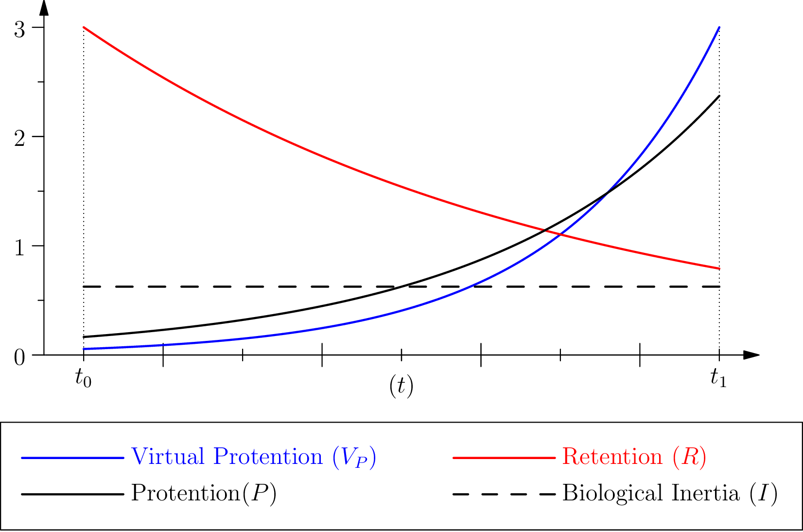
. This means that, in this condition, the vicinity of the virtual event is where the effect of protention is important, see figure 2.
It is crucial, however, to understand that protention, for example in the case of a cognitive situation, is not empirically associated with a change of behaviour, but with the speed of this change of
behaviour. This suggests a way to approach these quantities empirically by a comparison of the reaction time between situations where the event associated with retention (at time
) occurs and when it doesn’t: in the first case, a more sudden change is then to be expected close to the the expectation time
. Alternatively, the situation when the event at time
occurs but where the event (at time
) doesn’t occur allow to evidenciate the presence of protention and to see a part of its effects, it is the case of amoeba in Saigusa et al. 2008. However, in
many situations, the effect of protentional action will consist in a “sensibilization” to the virtual stimuli with the preparation of a response. This may lead to no behavioural change when the virtual stimuli doesn’t happen, but leads
to a change of organization associated with the preparation of the response (including at the sensory level) and possibly to a greater sensitivity to noise.
2.4 Global protention
One may wonder when protention is maximal for a given individual. In our approach, the first possible answer is given by looking at the diagram in figure 2: this quantity is maximal close to . However, we can refine the question (and the answer) by looking at the global amount of protention along the intended interval . As protention is both variant and contravariant in the size of (see definition 3), this question has a non-obvious answer.
For this purpose, we define the notion of global protention, which is the sum (the integral) of protention over time, between and .

This quantity has a maximum for , this maximum is a compromise between the need to give the protention time to have effect (covariant dependence on the size of ) and the need to have instants in that are close both to and (contravariance). This result means that there is a specific duration between the past event and the future event which optimize the protentional effects. This seems to be consistent with the results in Saigusa et al. 2008, since these authors found that a specific value of the delay (in our notation) leads to a greater protentional effect, that is the functional dependency on this interval of time has a maximum (a non-obvious fact). In section 3 we will go back to the relevant ratio .
3 Biological inertia
Consider now a relaxation phenomenon in physics, typically given by . If time is given, one may decompose as
The coefficient, not depending on , that is , is the “residual” at time and it may be understood as a form of “inertia” of the intended relaxed quantity (for example, it corresponds to “what remains” at time of a compound which decay with characteristic time ). This coefficient is constant in the interval and decreases for increasing .
In eq. (4) one has the following factors that do not depend on :
The first exponential term corresponds to a physical inertia, let’s call it . Then, we can consider that the other coefficient of protention represents a biological inertia, in the interval , depending on the biological constants , , and :
In other words, protention in eq. (4) may be considered as a product of a function of time , , modulated by constants and characteristic times, of a physical inertia and of a “biological inertia” . This last coefficient is also independent of , but depends on the specific organism by the various indexed constants.
The physical inertia represents the “passive” decay of a physical relaxation phenomena, which makes a perturabtion disappear during the return to equilibrium. On the contrary, the biological inertia coefficient is to be understood as a capacity to “carry over” the protensive effect. Their names are freely inspired by the inertial mass as a coefficient of acceleration (thus and very informally, biological inertia would be the biologically pertinent coefficient of protention). In section 4, by references and a discussion, we will say more about this new concept. First a few technicalities.
We have to check whether our definitions depend on the specific reference we choose. That is to say if a time origin change:
changes the way we split in three parts, in equation 4. It it then straightforward to see that:
This means that each of this quantities have a sound biological meaning.
Inertia introduces a coefficient which is independent of and is, in general, much smaller than (and always smaller than ). This coefficient contributes to the dependence of in function of . In particular, it contributes in an essential manner to the decrease of the protention according to the temporal distance.
3.1 Analysis

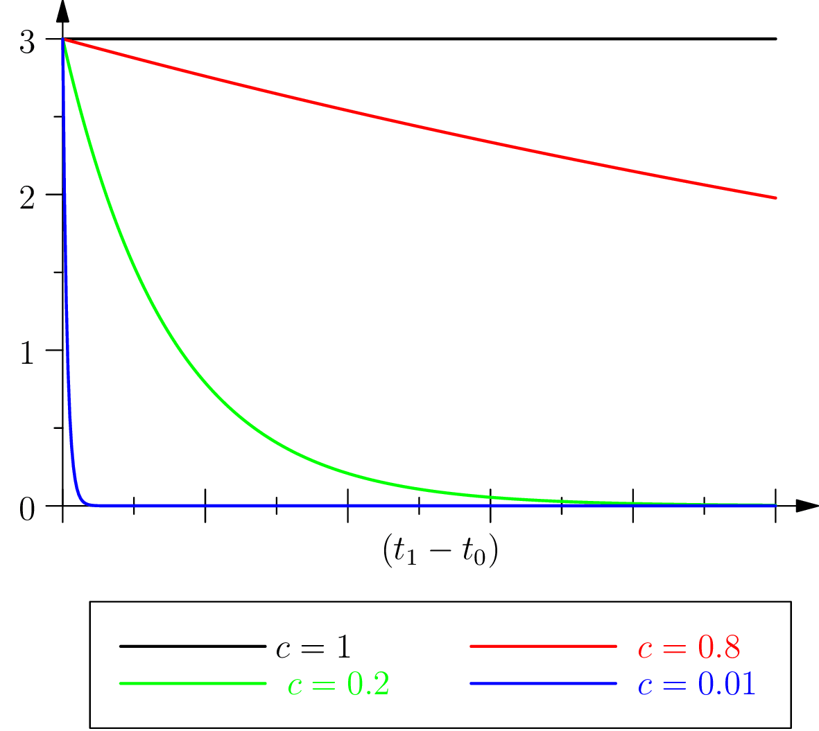
In order to better understand the sense we attribute to this “inertia” of living phenomena, given our preceding remark regarding orders of magnitude respective of characteristic times, we may focus on the ratio of figure 3, that is on such that . We consider and rewrite in the equivalent form:
Then has the form of a “long term retention” if or a “short term retention” if . Conversely, and maybe even more intuitively, inertia can be also interpreted (by writing and eliminating this time ) as a “long term virtual protention” :
Biological inertia would then be both an extended retention, eq. (15), and a virtual protention, eq. (17), which are both independent of the time of the action: in fact, it depends only on the instants that are relevant to the event retained and occurring in or which is the object of an expectation (protention towards ). It is therefore an inertia which “carries over” the life form from towards , by the preservation of its own structure and its relationship with the environment (see section 4).
The case
It can be observed that in the case where the characteristic retention and virtual protention times are equal ( where the from the equation above is equal to 1), the protention becomes and is therefore independent of the present observation time . This, of course, within the interval between the moment of the occurrence of the event in question and the moment where it is mobilized again (since we still have ). But then, according still to hypothesis , one has , with . Thus, when , only inertia is present in protention.
We can also note this situation by considering that if the observation time is close to the instant of the occurrence of the event (recent retention), then the temporal interval for a virtual protention, ), increases; conversely, if time is far from (remote retention), the temporal interval involved in this virtual protention and within which the latter plays its role (the future of the observation moment ) diminishes in importance, given of course that the protention as such remains independent of , in this case.
These remarks are meant to highlight the fact that, in the latter case, the intensity of the protention remains invariant, whereas the duration upon which virtual protention takes place — the future of — can change in size: .
4 References and more justifications for biological inertia
We have come to propose a mathematical notion of biological inertia through an apparently arbitrary play of symmetries and calculations, of which we would now like to better explain the meaning and the objectives. To emphasize the importance of the concept, but without wanting to make excessive and uncontrolled analogies with immensely illustrious precedents, let’s note that modern physics started off with a good analysis of inertia, as a “pursuing a state” without aim nor teleology: Galilean inertia[3].
In biology, this notion can already be found, although rarely, under various forms. For Vaz and Varela 1978 “the lymphoid system has an inertia, which resists attempts to induce sudden and profound deviations in the course of events”. So this is a weak notion of inertia, close to the “persistence” of structural stability. Likewise, we could talk about inertia in the case of the notion of “dynamic core” presented in Edelman and Tononi 2000, because it also refers to the continuity/persistence of individuation (see also Le Van Quyen 2003). This theme is also used by Varela 1997, where the term of inertia appears also in the attempt to grasp the “force”, specific to any organism, enabling its “bringing forth of an identity”.
In our approach, which is inspired by the methods of physics without identifying with it, we firstly define retention by a relaxation function, which is a physical notion — which can even be considered as adequate to describe the “memory” to which some often refer in relation to certain physico-chemical activities. Virtual protention is given then by a temporal symmetry, modulo some adjustment coefficients; this notion, which has no analogy in physics, is by this, and at least, the “projective” reflection of retention. Protention follows, as a linear combination of these two values, in function of time. Then, by a simple algebraic device, we separate the part containing the temporal variable from the functional definition: what remains is a constant, a function of all other parameters (characteristic times, specific constants, interval range), which we called biological inertia. As we pointed out, when retention and protention have the same characteristic times , inertia coincides with protention. We would then say that this is the simplest situations from a cognitive viewpoint: the organism can only anticipate by means of inertia. In any case, the proposed notion of inertia appears to clearly specify the informal idea of “bringing forth of an identity”, with the reference to retention and to protention, at the minimal cognitive level.
But why would this inertia not simply correspond to the fact of following a geodesic trajectory, like in physics? Some will say that the amoeba, the paramecium, etc., follow a gradient in the same way that a physical object follows the trajectory dictated by the Hamiltonian (through the principle of least action). It may appear that such is the case in in vitro experiments where, within a highly purified environment, the unicellular organism is exposed to one or two very specific gradients (chemical, thermal …). On the other hand, in an in vivo situation, in the ecosystems preferred by such animalcules (and which are very polluted, from our standpoint) they must “arbitrate” between qualitatively different stimuli: several physico-chemical gradients, an edible and close bacterium that is not too large, another smaller one, etc. Now the paramecium, say, appears to “learn” (see [Mislin, 2004]), that is, it enjoys at least retention, which contributes to protention (and, after reading Mislin and references, one could posit for it , or even [4]. And it is difficult to conceive of learning without error, or without several attempts and without the memory of these attempts (retention), even if such memory is extremely rudimentary. The subsequent action is therefore one among many possible ones, from the standpoint of the ecosystem, because it also depends on the specificity of individual retention (experience). Among these many possible trajectories, the one it follows has only to be compatible with the ecosystem. No gradient or physical geodesic is adequate to describe this plurality of possibilities of evolution, phylogenesis, ontogenesis and of action, which also depends on the specificity, hence on the history, of the species or of the individual (retention and biological inertia). Our modest inertial attempt tries to do this, in a way that is as preliminary as mathematically simple.
We can interpret the growth of as a greater cognitive “complexity”. It appears that the protention, when , must account for more “experience” in order to achieve the objective of the action; it depends upon a greater amount of lived and retained history, and hence on a greater specificity (individuality) of the living object. So it better participates to the incessant process of individuation, which is a play between the richness of retention and the diversity of possible future trajectories.
Another way to associate a growth of complexity to the growth of , is to consider cases where the global protention is constant. Then the increase of means that protention is more localized near , with the same global effect. Then this situation is more “complex”, since the preparation to the virtual event occurs when it is closer (and the organism must be “quickly ready”). In this case, it is easier for it to protend another event , with between and , since the organism is not yet fully focused on (the grows very slowly “for long” and fastly increases only close to ). This situation allows the organism to have longer times of correlation: during the early part of these extended protentional activities, it may prepare also for other events.
5 Towards human cognition. From trajectory to space: The continuity of the cognitive phenomena
The continuity of space-time, which the mathematics of continua proposes and structures in a remarkable way, from Euclid to Cantor, follows — and does not precede — the continuity of a figure, of a contour or of a trajectory. Euclidean geometry is not a geometry of space, it is a geometry of figures, with continuous edges, constructed by means of ruler and compass and submitted to translations and to rotations. It is much later, with Descartes, that geometry finds its constitutive environment in an abstract space, underlying and independent from the figures which evolve within. The analytical reconstruction of Euclidean geometry will follow, by means of this ideal framework, an algebraico-geometrical continuum, organized in Cartesian coordinates. Then, since Cantor, we have a fantastic reconstruction of the underlying continuum, a possible one, though (see Lawvere and Bell for an alternative topos-theoretic approach, with no points, Bell 1998).
Let’s now try to grasp a possible constitutive path or even a cognitive foundation of this phenomenal continuum which is the privileged conceptual and mathematical tool for the intelligibility of space, on the basis of our analysis of retention and of protention.
The recent analyses of the primary cortex (see Petitot 2008 for a survey) highlight the role of intracortical synaptic linkages in the perceptual construction of edges and of trajectories. Neurons correlate themselves locally, along “association fields” (Field 1987; Field, Hayes, and Hess 1993) composed of smooth (differentiable) curves that “are grouped toghether only when alignement fails along particular axes” Field, Hayes, and Hess 1993. These neurons are sensitive to “directions”: that is, they activate when detecting a direction, along a tangent. Then they (pre-)activate other neurons in the association field (they prepare in advance the spike which is not yet fired). This preactivation of associated neurons is, in our view, a component of the protensive activity. Then, neuronal activation follows a specific direction which (re-)constructs the pertinent line, Petitot 2008.
Thus, the continuity of an edge or of a trajectory is constructed by “gluing” together fragments of the world, in the precise geometrical (differential) sense of gluing. In other words, we force by continuity the unity of an edge by relating neurons which are pre-associated and are, locally, along particular axes.
This phenomenon participates in the retention and the protention of a non-existing line, a trajectory say, by “integrating”, in the mathematical sense, the tangents that are locally associated in the field. The related inertial phenomena of the activation/deactivation of neurons may be one of its constitutive elements, with inertia as a coefficient of protention. The retention of occular movements or saccades which follow a moving body, an edge, should also be quoted: this retentive/protensive phenomenon originates in the muscles enabling the saccades or in the neurons managing them. As for the case of protention, in particular, there are protentional displacements in the receptor field of the cortical neurons that precede the saccades (Berthoz 2002). The brain prepares itself and anticipates a moving object, of which the movement is perceived following an occular saccade, or of which the trajectory or edge is perceived by running the eye along or over it. This is, in our view, the keystone of a fundamental protentional activity.
Now, we propose the following conjecture. First, the World is not continuous, nor discrete: it is what it is. Since Newton and Cantor, by continuous tools, or, now, in Quantum theories and Topos Theoretic approaches, we mathematically organized it in various ways, possibly over different “backgrounds”. In our view, the phenomenal continuity of trajectories, of an edge, is due to the retention of that trajectory, edge, scanned by the eye, which is “glued” with the protention by the very unit of the cerebral and global physiological activity (the vestibular system, for example, has its own retention and inertia).
In the case of contours, the specific saccades along the direction of movement or towards the extreme of a reconstructed segment (for example in Kanizsa triangles, see Petitot 2008) stimulates a specific activation in the association field (a specific connection between neurons in the field).
It would then be this “gluing” — a mathematically solid concept (at the center of differential geometry, of which Riemannian geometry is a special case) — that entails the cognitive effect which imposes continuity upon the world: the image of the object and of its past position is reassembled (glued by the conjunction of protention and retention) with that of the object and of its expected position or a contour is made continuous even when non existing (as in Kanizsa illusions). We could indeed imagine that an animal with no fovea (the part of the eye which enables a follow up of a target by a continuous focus), a frog for example, and which takes spaced out snapshots of an object in movement would not have the impression of a continuous movement in the way in which we, the primates, “see” it.
By measuring relaxation and (pre-)activation times of associated neurons it should be possible to quantify our coefficients in these specific phenomena. Inertial coefficients in particular would yield different values according to the different protentional capacities in different species (frogs for example may have no inertia w.r. to these phenomena, if our understanding above is correct).
So the continuity of a trajectory or of an edge is, in our opinion, the result of a spatio-temporal reassembling of the retentions and protentions that are managed by global neural activity in the presence of a plurality of activities of such type (muscles, vestibular system …but also the differentiable continuity of the movement or gesture participates by means of its own play of retention/protention). In short, by a cognitive process of glueing, we attribute continuity to phenomena which are what they are (and which a frog surely sees quite differently). Then, by a remarkable conceptual and mathematical effort having required centuries, we have even come to theorize, as abstract lines, surfaces and their edges, first, and then even the continuity of environing space, as the background of these structures. And this is the consequence, we believe, not the cause of the cognitive/perceptive continuity of the movement and of the gesture, which is instead grounded on the unity of protention and retention (note that, in this perspective, the continuity of an edge would also be the continuity of a movement: the movement of the saccade or of the hand caressing it, both retained and protended).
Let’s note that, in our attempt towards spatialization of time for living phenomena, in this paper and in Bailly, Longo, and Montévil 2011, — a spatialization which, although schematic, should contribute to its intelligibility — we have proceeded, in this section, along the opposite approach: a sort of temporalization of space. Its apparent continuity would be the result of a cognitive activity on time, the extended present obtained by rentention and protention.
Acknowledgements We would like to thank the anonymous referee for his/her critical comments and suggestions. Longo’s papers are downloadable from http://www.di.ens.fr/users/longo/.
References
- Bailly, F., and G. Longo. 2008. “Extended critical situations: the physical singularity of life phenomena.” Journal of Biological Systems 16 (2): 309. doi: 10.1142/S0218339008002514. (Cited on pages 3, 5).
- _________. 2009. “Biological organization and anti-entropy.” Journal of Biological Systems 17 (1): 63–96. doi: 10.1142/S0218339009002715. (Cited on page 3).
- _________. 2011. Mathematics and the natural sciences; The Physical Singularity of Life. London: Imperial College Press. (Cited on page 3).
- Bailly, F., G. Longo, and M. Montévil. 2011. “A 2-dimensional geometry for biological time.” Progress in Biophysics and Molecular Biology 106 (3): 474–484. issn: 0079-6107. doi: 10.1016/j.pbiomolbio.2011.02.001. (Cited on pages 3, 31).
- Bak, P., C. Tang, and K. Wiesenfeld. 1988. “Self-organized criticality.” Physical review A 38 (1): 364–374. doi: 10.1103/PhysRevA.38.364. (Cited on page 5).
- Bell, J. 1998. A Primer in Infinitesimal Analysis. Cambridge U.P. (Cited on page 30).
- Berthoz, A. 2002. The Brain’s Sense of Movement. Harvard U.P. (Cited on pages 4, 30).
- Botzung, A., E. Denkova, and L. Manning. 2008. “Experiencing past and future personal events: Functional neuroimaging evidence on the neural bases of mental time travel.” Brain and Cognition 66 (2): 202–212. doi:10.1016/j.bandc.2007.07.011. (Cited on page 35).
- Edelman, G.M., and G. Tononi. 2000. “Reentry and the dynamic core: neural correlates of conscious experience.” In Neural Correlates of Consciousness: Empirical and Conceptual Questions, edited by T. Metzinger, 139–151. MIT Press. (Cited on page 28).
- Field, D.J. 1987. “Relations between the statistics of natural images and the response properties of cortical cells.” Journal of the Optical Society of America A 4 (12): 2379–2394. doi: 10.1364/JOSAA.4.002379. (Cited on page 30).
- Field, D.J., A. Hayes, and R.F. Hess. 1993. “Contour integration by the human visual system: Evidence for a local association field.” Vision Research 33 (2): 173–193. doi: 10.1016/0042-6989(93)90156-Q. (Cited on page 30).
- Kauffman, Stuart A. 1993. The origins of order: Self organization and selection in evolution. Oxford university press. (Cited on page 5).
- Le Van Quyen, M. 2003. “Disentangling the dynamic core: a research program for a neurodynamics at the large-scale.” Biological Research 36:67–88. doi: 10.4067/S0716-97602003000100006. (Cited on page 28).
- Lindstedt, S.L., and W.A. Calder III. 1981. “Body size, physiological time, and longevity of homeothermic animals.” Quarterly Review of Biology: 1–16. doi: 10.1086/412080. (Cited on page 5).
- Longo, G., and M. Montévil. 2011. “Protention and retention in biological systems.” Theory in Biosciences 130 (2): 107–117. issn: 1431-7613. doi: 10.1007/s12064-010-0116-6.
- Misslin, R. 2003. “Une vie de cellule.” Revue de Synthèse 124 (1): 205–221. doi: 10.1007/BF02963405. (Cited on page 4).
- Nicolas, F. 2006. “Quelle unité pour l’œuvre musicale?” In Les mathématiques, les id ées et le réel physique. Paris: Vrin. (Cited on page 2).
- Nicolis, G., and I Prigogine. 1977. Self-organization in non-equilibrium systems. New York: Wiley. (Cited on page 5).
- Perfetti, C.A., and S.R. Goldman. 1976. “Discourse memory and reading comprehension skill.” Journal of Verbal Learning and Verbal Behavior 15 (1): 33–42. issn: 0022-5371. doi: 10.1016/S0022-5371(76)90004-9. (Cited on page 2).
- Petitot, J. 2008. Neurogéomé trie de la vision. Ed de l’École Polytechnique. (Cited on pages 30 sq.).
- Saigusa, T., A. Tero, T. Nakagaki, and Y. Kuramoto. 2008. “Amoebae anticipate periodic events.” Physical Review Letters 100 (1): 018101. doi: 10.1103/PhysRevLett.100.018101. (Cited on pages 4, 16, 20).
- Savage, V.M., J.F. Gilloly, W.H. Woodruff, G.B. West, A.P. Allen, B.J. Enquist, and J.H. Brown. 2004. “The predominance of quarter-power scaling in biology.” Ecology 18:257–282. doi: 10.1111/j.0269-8463.2004.00856.x. (Cited on page 5).
- Suzuki, M., K. Kaneko, and S. Takesue. 1982. “Critical Slowing Down in Stochastic Processes. I.” Progress of Theoretical Physics 67 (6): 1756–1775. doi: 10.1143/PTP.67.1756. (Cited on page 6).
- Szpunar, K.K., J.M. Watson, and K.B. McDermott. 2007. “Neural substrates of envisioning the future.” Proceedings of the National Academy of Sciences 104 (2): 642. doi: 10.1073/pnas.0610082104. (Cited on page 35).
- Van Gelder, T. 1999. “Wooden iron? Husserlian phenomenology meets cognitive science.” In Naturalizing Phenomenology: Issues in Contemporary Phenomenology and Cognitive Science, edited by J. Petitot, F.J. Varela, B. Pachoud, and J.M. Roy, 245–265. Stanford U. P. (Cited on page 2).
- Varela, F.J. 1997. “Patterns of life: Intertwining identity and cognition.” Brain and Cognition 34 (1): 72–87. doi: 10.1006/brcg.1997.0907. (Cited on page 28).
- _________. 1999. “The specious present: A neurophenomenology of time consciousness.” In Naturalizing phenomenology: Issues in contemporary phenomenology and cognitive science, edited by J. Petitot, F.J. Varela, B. Pachoud, and J.M. Roy, 266–314. Stanford U. P. (Cited on page 2).
- Vaz, N.M., and F.J. Varela. 1978. “Self and non-sense: an organism-centered approach to immunology.” Medical Hypotheses 4 (3): 231–267. doi: 10.1016/0306-9877(78)90005-1. (Cited on page 28).
- Wildman, D.M., and M. Kling. 1978. “Semantic, syntactic, and spatial anticipation in reading.” Reading Research Quarterly 14 (2): 128–164. (Cited on page 2).