Ecological models for gene therapy. I. Models for intraorganismal ecology

Ecological models for gene therapy 1: models for intraorganismal ecology

Arnaud Pocheville ⋅ Maël Montévil

Abstract

In this paper, we discuss the perspective of intra-organismal ecology by investigating a family of ecological models. We consider two types of models. First order models describe the population dynamics as being directly affected by ecological factors (here understood as nutrients, space, etc). They might be thought of as analogous to Aristotelian physics. Second order models describe the population dynamics as being indirectly affected, the ecological factors now affecting the derivative of the growth rate (that is, the population acceleration), possibly through an impact on non-genetically inherited factors. Second order models might be thought of as analogous to Galilean physics.
In the joint paper, we apply these ideas to a situation of gene therapy.

Keywords: Intra-organismal ecology  $\cdot$ niche construction  $\cdot$ ecosystem engineering  $\cdot$ non-genetic inheritance  $\cdot$ inertial dynamics

Introduction

The organism can be seen as a biome, composed of organs that are ecosystems where are played ecological and evolutionary drama Kupiec and Sonigo (2003).

This perspective draws back to the speculations of Roux (1881) and Weismann (1904)^[1]) on selection occurring inside the organism. More recently, eco-evolutionary processes between cells within an organism have been considered, both to explain the existence of protection mechanisms against the proliferation of cancer cells within an organism Cairns (1975); Nowak et al ( 2003), to predict the spread of resistant phenotypes within cell populations during cancer treatments Nowell (1976);  Merlo et al (2006), to describe intra-host dynamics of infectious diseases or cancers as predator-prey interactions between viruses and the immune system Nowak and May (2000); Merlo et al (2006)^[2], or to apply the neutral theory of biodiversity Hubbell (2001) to gut or skin flora communities (e.g. Turnbaugh et al (2007); Roth and James (1988,  1989)).

This paper takes place in such an intra-organismal eco-evolutionary perspective. The topic we are interested in is the study of a gene therapy. Gene therapy aims at correcting a physiological dysfunction whose origin is the inadequate expression of a defective gene. In practice, patient cells are genetically modified in vitro by inserting a given gene, and then re-injected to the patient, with the aim that these modified cells replace the resident cells, or at least that they durably persist within patient’s body: that is, that cells be successfully engrafted Aiuti and Giovannetti ( 2003); Cavazzana-Calvo et al (2005). From an ecological point of view, the prospective replacement of a cellular strain by another is similar to a competitive exclusion or a drift, while modification of the cellular environment, for instance by producing a missing enzyme, is similar to ecosystem engineering Jones et al (1994) or, in other terms, to niche construction (Odling-Smee et al ( 2003), chap.5)^[3]. Successful or unsuccessful engraftment qua species invasion will then depend on the details of the ecological interaction Gonzalez et al ( 2008). The aim of the present work is to determine the conditions of successful engraftment.

To this aim, we will study a family of ecological models describing the dynamics of cell populations within an organism. In the first part, we will present the family of models of competition between cells in the general, non-pathological, case. This will enable us to more easily discuss those aspects of the models that are not limited to the particular case of gene therapy.

General model of cell population dynamics

We consider that cells proliferate inasmuch as limiting constraints enable them to. More specifically, we will assume here that the population dynamics directly depends from a limiting factor $\phi \left(t\right)$. $\phi \left(t\right)$ may, in principle, be any kind of quantity that is extensive (i.e. proportional to the size of the system) and restricts the tendency of cells to proliferate: available space, fluxes of nutrients, oxygen, growth factors, etc. In the following models, we will not specify $\phi \left(t\right)$ ’s dynamics, in particular, we will consider that $\phi \left(t\right)$ is not modified by cell populations (e.g. there is no stock or consumption dynamics), and that it is determined by factors that are external to the considered organ. Thus, $\phi \left(t\right)$ forces^[4] the dynamics. This hypothesis could be relaxed by modeling $\phi \left(t\right)$ as a prey within a predator-prey system, but this generalization is not necessary at this step.

1 First order model

We consider that the limiting factor $\phi \left(t\right)$ is instantaneously equitably shared among cells. This hypothesis is similar to the ratio-dependence hypothesis in predator-prey models (Arditi and Ginzburg ( 1989); Akçakaya et al (1995). The model is assumed to be valid only when the number $N$ of cells is large enough, that is, the model is valid when the considered factors $\phi \left(t\right)$ are limiting. The per capita growth rate $r$ increases instantaneously, linearly with the available quantity of limiting factor by cell: we thus consider a situation where doubling both the limiting factor and the population will not change the per capita growth rate by cell. Cells undergo a constant intrinsic mortality $m$.

$$r=\frac{dN}{Ndt}=\frac{a\phi }{N}-m$$

(1)

where $A$ is a scale constant.

Equation 1 admits one (stable) equilibrium:

$$N^{\ast }=\frac{a\phi }{m}$$

---

---

The system relaxes towards the equilibrium with a characteristic time $\tau =1∕m$ (figure 1). This equilibrium requires $\phi \left(t\right)$ to have a sufficiently slow dynamics to allow us to consider the limiting factor as locally constant. We can then consider that at the scale of $\phi \left(t\right)$ variations the system follows its equilibrium value in function of $\phi \left(t\right)$ :

$$N\left(t\right)\simeq \frac{a\phi \left(t\right)}{m}$$

From then on, we consider only the case where $\phi \left(t\right)$ is constant at the scale of $N\left(t\right)$ variations. To ease reading, we will write it $\phi$.

2 Second order model

We now turn to a different type of modeling, following the works of Ginzburg and colleagues on demographic inertia Ginzburg et al (2004). We consider that the per capita growth rate now shows a certain inertia (comparable to inertia in Newtonian physics) that is perceptible at the scale of population dynamics. Put it differently, we will not separate the time-scales of the per capita growth rate dynamics and of the population dynamics.

From the biological point of view, such an inertia in the per capita growth rate can result from a dynamics in cell quality (e.g., available amount of intracellular resources or organization quantity, sensu Bailly and Longo (2009)). Then, if environmental conditions worsen, intracellular resources lead to a delay in the demographic response; conversely if living conditions get better the cells first rebuild their intracellular resources before their demographic parameters (division and mortality) get affected. Individual quality can also be transmitted to offspring, a phenomenon known in ecology as maternal effects (e.g. Mousseau and Fox (1998)).

In this model, it is the change of the per capita growth rate that depends on the per capita limiting factor $\phi$, times a given constant $A$. In the absence or lack of the limiting factor, the per capita growth rate decreases at a rate $m$ ( $m$ typically models the amount of the limiting factor required to sustain proliferation, for example the consumption of oxygen or nutrient) We can now write the equation of demographic acceleration:

$$\frac{\mathit{dr}}{\mathit{dt}}=\frac{a\phi }{N}-m$$

(2)

The model is formally similar to the first order model, but notice that the dimensionality and the meaning of the variables has now changed. The equilibrium of equation 2 results when $r=0$ and $N^{\ast }=a\phi ∕m$. The equilibrium is stable.

2.1 A note on the analogy with physics

In this model, demographic factors ( $\phi$ and $m$) impact the acceleration $dr∕dt$ and not the speed $r$ of demographic change. This conceptual change is worth discussing at some length, as it will enable to reveal some of the deep theoretical assumptions that lie behind modeling choices. This will lead us to discuss ideal, default states in population dynamics, with the proviso that the aim of a theory is to describe the deviations from the default state ( e.g., zero force case).

According to equation 2, in the idealized case where $\phi =m=0$, the population grows (or decreases) at a constant pace that depends on initial conditions, which is equivalent to the uniform straight movement of a body on which no force is exerted in Newtonian physics. By contrast, the first-order, non-inertial model (equation 1) is comparable to Aristotelian physics, where the absence of any factor modifying the dynamics results in zero speed (demographic stasis).

Our interpretation of demographic inertia departs from Ginzburg’s here Ginzburg et al (2004) (chap.6), who consider that the default state of dynamics is the absence of limiting factors (i.e. $r=r_{max}$). With Ginzburg’s interpretation, the default dynamics (equivalent to the straight uniform movement) depends on a biological property ( $r_{max}$), and not from initial conditions (by contrast with the straight uniform movement, where the speed depends on the initial speed $v\left(0\right)$ and not on the properties of a physical body such as its mass). Ginzburg’s interpretation of what the default dynamics should be is similar to Lotka’s (1925) in his first order equation $\mathit{dN}∕\mathit{Ndt}=r\left.1-N∕K\right)$, where when $N$ is small in comparison with $K$, limiting factors ( $K$) do not impact the dynamics and the speed $dN∕Ndt$ is given by the maximum per capita growth rate.

By contrast, we consider here that the metabolism $m$ should count as a factor impacting the acceleration $dr∕dt$, and we should accept to ignore metabolism to produce an idealization comparable to Newtonian idealization. In this case the idealized dynamics is given by the initial condition $r\left(0\right)$ and not the property $r_{max}$.

Contrary to Newtonian physics however where the default state is general, the idealized equation 2 where all factors are put to zero can make sense only in very special cases where cell quality is fully heritable during divisions (e.g. some environment sensitive epigenetic marks), that is, it does not hold for intracellular resources that are shared among daughter cells. Below we will consider the impact of resource sharing among offspring, and see how it radically modifies the dynamics

2.2 Differences between inertial and non-inertial dynamics: accelerated death, overshoot

---

---

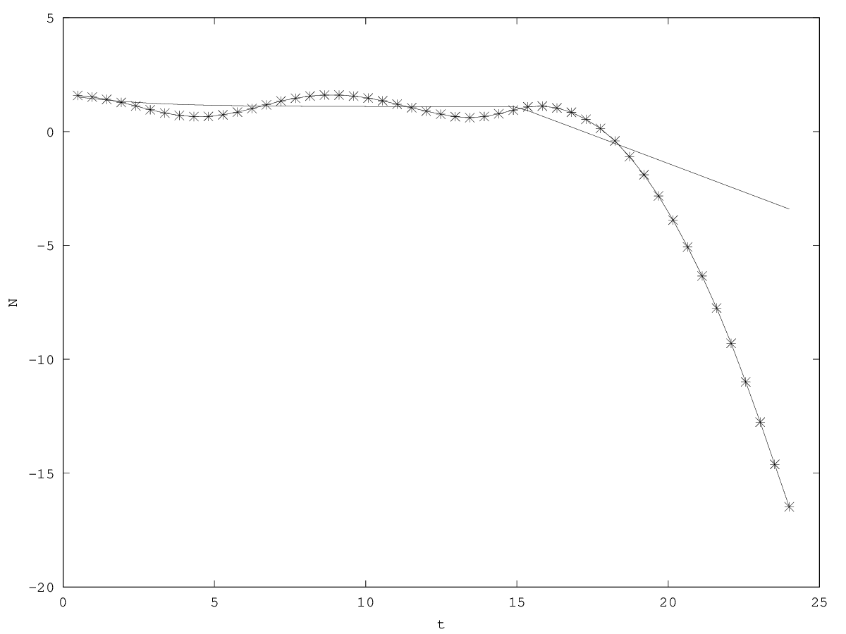
In the inertial model (equation 2), death is accelerated when the limiting factor is the strongest (i.e. set to zero): the per capita growth rate decreases and can tend towards $-\infty$ (that is, death rate tends to be instantaneous). By contrast, in the non-inertial model (equation 1), in the absence of the limiting factor the per capita growth rate remains constant (and negative: $\phi =0$ implies $r=-m$) (figure 2.2). At the level of organisms population dynamics, accelerated death is empirically observed Akçakaya et al (1988);  Ginzburg et al (1988).

---

---

---

---

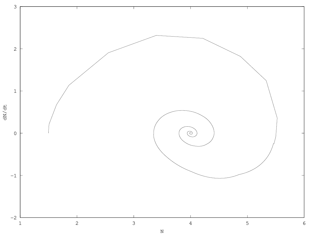
An inertial dynamics also allows to overshoot the demographic equilibrium value of the population (figure 2.2, figure 2.2). Overshoot leads to demographic oscillations around the equilibrium value with a pulsation $\sqrt{m}$, that is, a period $T=2\pi ∕\sqrt{m}$ (see appendix 5.3). In biological terms, metabolism accelerates the pulsation, which can be interpreted as an acceleration of biological time Bailly et al (2011).

2.3 Friction, antifriction

In the model described by equation 2, oscillations around the equilibrium value are neither damped nor amplified. Such a behavior is structurally unstable: small modifications of the model lead to the convergence toward stable equilibrium or to divergence May (1973); Nowak and May ( 2000).

From a biological point of view, oscillations are damped when good quality cells ( $r>0$) tend to waste their intracellular resources more and/or when poor quality cells ( $r<0$) spare their resources. Also, when cells share their resources during a division between daughter cells, there is a negative impact of $r$ on itself, through cell quality, which leads to oscillation damping. By contrast, oscillations would be amplified if good quality ( $r>0$) entailed a virtuous circle improving cell organization and quality, and poor quality ( $r<0$) entailed a vicious cycle leading to even more decreased $r$. Note that the environment can also have friction, forcing or resonance effects. We can capture this dynamical behavior whose causes are diverse with a simple phenomenological function that represents friction ( $f>0$) or antifriction ( $f<0$).

$$\frac{\mathit{dr}}{\mathit{dt}}=\frac{a\phi }{N}-m-fr$$

(3)

Equation 3 cancels out when $r=r^{\ast }$ :

$$r^{\ast }=\frac{1}{f}\left.\frac{a\phi }{N}-m\right)$$

$r^{\ast }$ corresponds to the limiting speed due to friction ( $f>0$, $r^{\ast }$ is a stable equilibrium) or antifriction ( $f<0$, $r^{\ast }$ is an unstable equilibrium).

In particular, in the case of a free fall ( $N=\infty$ or $\phi =0$) with friction ( $f>0$), $r$ reaches a maximal value: $r^{\ast }=-m∕f$. In this case, the per capita growth rate is given by two intrinsic cellular properties, metabolism and friction. This limiting speed is analogous to the limiting speed of a body in free fall in a medium with non-null viscosity, which is also given by medium and body properties.

Ginzburg et al (2004) p90 also modeled population dynamics with a second order equation (that is, with $dr∕dt$) with a phenomenological term of friction. However, the limiting speed (per capita) of a free fall in their model is proportional to $N∕N^{\ast }$, which is not a property of the cells^[5].

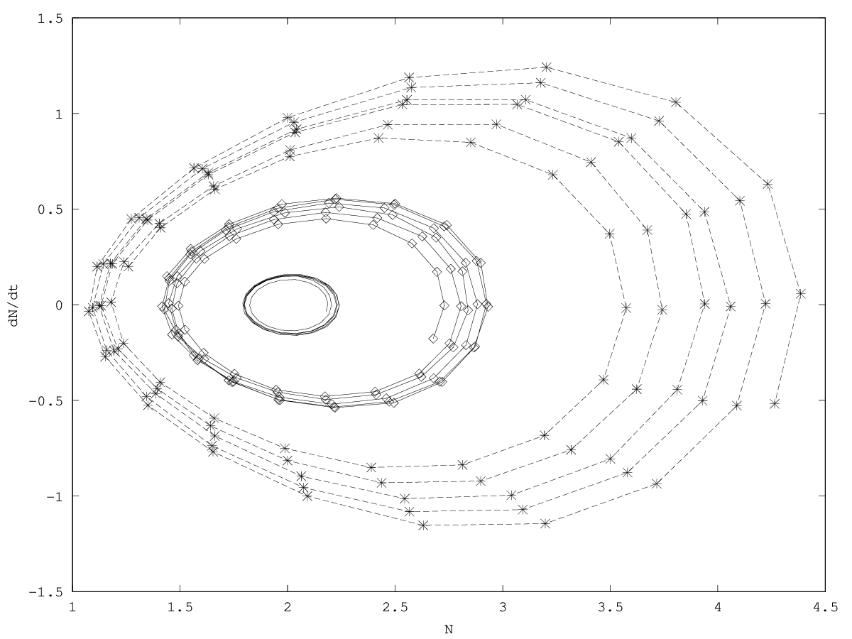
Close to the equilibrium, the system with friction ( $f>0$) can follow three different regimes depending on the sign of $\Delta =f^2∕4-m$ (figure 2.3 & 2.3, see calculations in appendix 5.3):

---

---

---

---

1. pseudoperiodical regime with damped oscillations ( $\Delta <0$): the pulsation is given by $\omega$:

   $$\omega =\sqrt{m-\frac{f^2}{4}}$$

   The period is given by $T=2\pi ∕\omega$. The relaxation time is given by $\tau$ :

   $$\tau =\frac{2}{f}$$

2. critical regime ( $\Delta =0$): the system shows no oscillations and relaxes with a characteristic time $\tau =2∕f$.
3. aperiodical regime ( $\Delta >0$): the systems returns to equilibrium with a relaxation time $\tau$:

   $$\tau =\frac{2}{f-2\sqrt{\frac{f^2}{4}-m}}$$

   Note that relaxation is slower than in the damped oscillation regime, because now friction also opposes to the return to equilibrium.

We will see how, from a theoretical point of view, the existence of friction in cell population dynamics can have therapeutic implications.

3 Model with two species

In this section we derive the models of sections 1.1 and 1.2 to describe the case of an interaction between two species (in our case, two cellular strains). These are the models we will use in the next part. Though we describe the dynamics from a general point of view in this section (that is, without making any symmetry assumption about the species in presence) we will be able to drastically reduce the number of parameters in the following part assuming that the cellular strains (genetically modified and non-modified) are identical in most respect.

3.1 First order model

We suppose that the two species interact in a competitive way via their dependency to the limiting factor $\phi$. We described the interaction by making a superposition hypothesis (i.e., of linear competition) comparable to the one used in the Lotka-Volterra interspecific competition model.

$$\begin{array}{lll}\hfill \frac{d{N}_1}{N_{1}dt}& =\frac{a_1\phi }{N_1+q_{2\to 1}{N}_2}-m_1& \hfill \text{(4)}\\ \hfill \frac{{dN}_2}{N_{2}dt}& =\frac{a_2\phi }{N_2+q_{1\to 2}{N}_1}-m_2& \hfill \text{(5)}\end{array}$$

$q_{i-j}$ describes the per capita effect of $i$ on $j$. The model is valid only if $q\ge 0$, that is, in the case of competition. If $q<0$, the interaction corresponds to facilitation and the hypothesis of superposition is not adequate anymore (we should then introduce for instance a reciprocal saturation term between $N_1$ and $N_2$).

---

---

The behavior of the system, and in particular the stability of the equilibra in the space of parameters is shown in figure 3.1. The system has three equilibria: two equilibria correspond to the loss of a least one species and reduce to the monospecific case, one corresponds to the coexistence between populations $1$ and $2$.

(a) $N_1^{\ast }=0$ and $N_2^{\ast }=a_2\phi ∕m_2$ ; or $N_2^{\ast }=0$ and $N_1^{\ast }=a_1\phi ∕m_1$.

(b) the equilibrium corresponding to coexistence is given by the couple $\left\{N_1^{\ast },N_2^{\ast }\right\}$, when $q_{21}{q}_{12}\ne 1$ :

$$\begin{array}{llll}\hfill N_1^{\ast }& =\left.\frac{1}{1-q_{21}{q}_{12}}\right)\left.\frac{a_1\phi }{m_1}-q_{21}\frac{a_2\phi }{m_2}\right)& \hfill & \\ \hfill N_2^{\ast }& =\left.\frac{1}{1-q_{21}{q}_{12}}\right)\left.\frac{a_2\phi }{m_2}-q_{12}\frac{a_1\phi }{m_1}\right)& \hfill & \end{array}$$

The equilibrium is a coexistence iff $N_1^{\ast }>0$ and $N_2^{\ast }>0$. There is never coexistence if $q_{21}{q}_{12}=1$, except in the particular case where $a_1∕m_1=q_{21}{a}_2∕m_2$. In this case, coexistence is neutral and the equilibrium is insensitive to the relative abundances of 1 and 2, as long as the equation $N_1+q_{21}{N}_2=a_1\phi ∕m_1$ is true.

3.2 Second order model

We similarly extend the second order monospecific model to the two-species case by doing the same assumptions about the competitive interaction between 1 and 2:

$$\begin{array}{lll}\hfill \frac{{\mathit{dr}}_1}{\mathit{dt}}& =\frac{a_1\phi }{N_1+q_{21}{N}_2}-m_1& \hfill \text{(6)}\\ \hfill \frac{{\mathit{dr}}_2}{\mathit{dt}}& =\frac{a_2\phi }{N_2+q_{12}{N}_1}-m_2& \hfill \text{(7)}\end{array}$$

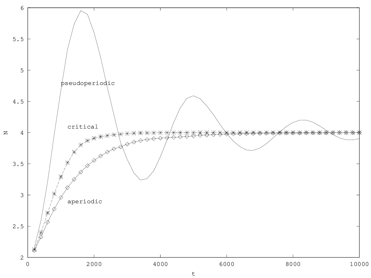
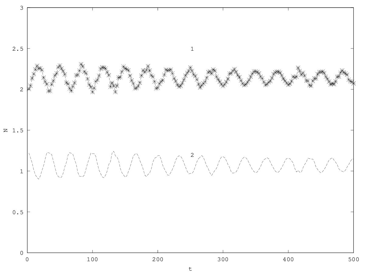
The equilibrium of this system obtains for the same equilibrium values than the first order system (steady $r$) and when the per capita growth rates are equal to zero ( $r_1=r_2=0$). The stability of the equilibrium is given by the sign of the highest eigenvalue (here noted $\nu$, the other eigenvalue being noted $\mu$, see appendix 5.5). When $\nu >0$ the fixed point $\left\{N_1^{\ast },N_2^{\ast }\right\}$ is unstable and one of the two populations is eliminated. If $\nu <0$, then $N_1$ and $N_2$ follow superimposed independent oscillations of pulsations $\sqrt{-\mu }$ and $\sqrt{-\nu }$ around the equilibrium value. The system does not show coupled oscillations (figure 3.2).

---

---

3.3 Second order model with friction

We now add friction to the two-species model:

$$\begin{array}{lll}\hfill \frac{{\mathit{dr}}_1}{\mathit{dt}}=\frac{a_1\phi }{N_1+q_{2\to 1}{N}_2}-m_1-f_1{r}_1& & \hfill \text{(8)}\\ \hfill \frac{{\mathit{dr}}_2}{\mathit{dt}}=\frac{a_2\phi }{N_2+q_{1\to 2}{N}_1}-m_2-f_2{r}_2& & \hfill \text{(9)}\end{array}$$

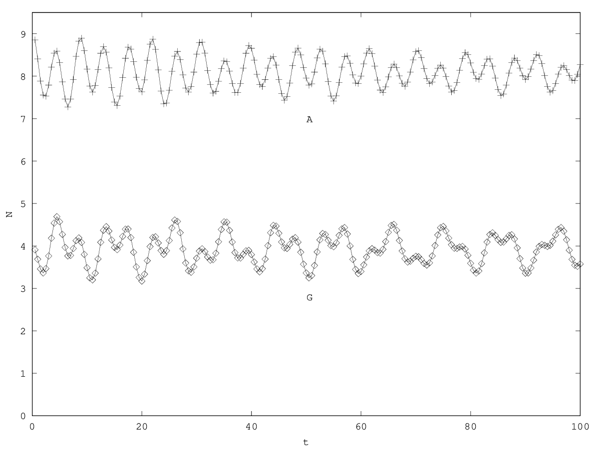
From then on, we will only consider cases where $f_1=f_2=f$. In this case, it can be shown that the conditions for local stability are not affected by friction (see appendix 5.6). In the stable case the dynamics corresponds to the linear superposition of two dynamics following equation 3, thus showing the same kind of behaviors. The main difference with the introduction of friction is that the system now tends towards its equilibrium, and near the equilibrium it relaxes towards equilibrium with damped oscillations.

4 Discussion

A model of population dynamics should exhibit three essential behaviors: decline in absence of resources, growth in non-limiting situations ( $r_{max}$)^[6], and the potential existence of a carrying capacity ( $N^{\ast }$) due to limiting factors (nutrients or space). These three behaviors can be biologically linked: for instance, an increase in mortality can affect both $r_{max}$ and $N^{\ast }$. In contrast, they can be biologically independent: for instance, if $N^{\ast }$ is due to limiting space, genetically modifying the cells can increase $r_{max}$ without affecting $N^{\ast }$.

It is impossible to represent the possible actions on these three independent behaviors with only two parameters (e.g., $a\phi$ and $m$ in our model, $r$ and $K$ in Lotka-Volterra), and it is impossible to represent a $N^{\ast }$ independent from $r_{max}$ with first order equations (Ginzburg 1992)^[7].

Under these constraints, and to favor parsimony which is essential to our application on gene therapy (next section), we have sacrificed the behavior of the population far from the $N^{\ast }$ (i.e., we did not introduce any $r_{max}$). An alternative choice would have been to use the logistic equation in Verhulst’s (1838) form:

$$\frac{\mathit{dN}}{\mathit{Ndt}}=a-\mathit{bN}$$

or in the version of Lotka (1925):

$$\frac{\mathit{dN}}{\mathit{Ndt}}=r\left.1-\frac{N}{K}\right)$$

We did not choose this model for the following reasons:

1. The difficulty of interpreting the parameters Olson (1992). First, $a$, or $r$, both represent $r_{max}$ and have an impact on the density-dependence ( $N^{\ast }=a∕b$ in Verhulst’s equation and thus depends on $r_{max}=a$ ; conversly, $N^{\ast }=K$ and is independent from $r$ in Lotka’s equation but now the density parameter, that is, the amount to which the population is sensitive to itself, is $r∕K$). Second, $K$ should not be interpreted as a carrying capacity but as an equilibrium value Berryman ( 1992). In other terms, in the logistic equation the inflexion point is a center of symmetry between growth when the population is small, and growth near the equilibrium, which does not seem to have any obvious biological basis Winsor (1932).
2. The unrealistic form of the density dependence Getz (1996), when $N\ll N^{\ast }$ McCarthy (1997); Courchamp et al (1999);  Etienne et al (2002); Kent et al (2003), but also when $N\gg N^{\ast }$ : in this case the per capita death rate is proportional to the ratio $N∕N^{\ast }$, and not to a property of the biological system in the absence of resources (death by food shortage for instance). This behavior comes from the fact that Verhulst’s equation is a truncated Taylor series. We find this same behavior in the inertial model of Ginzburg et al (2004) p90 which has the same form (but at the second order).

We have chosen here to model the dynamics for situations where $N$ is not far from $N^{\ast }$. The rationale for this hypothesis comes from our interest in modeling cell populations within an organism (see companion paper), that can be supposed to undergo only small or slow variations because of constraints posed by the organism. We have privileged a density-dependence that is less abrupt (sensu Getz (1996)) than the one of the logistic equation when $N\gg N^{\ast }$, in particular, we have priviledged a free fall speed that is a property of the individuals, and not a function of the distance between $N$ and $N^{\ast }$. Such attention to the form of density dependence could turn out to be crucial in niche construction cases where the modification of the $N^{\ast }$ is the focal behavior (Odling-Smee et al (2003), Pocheville (2010) chap.2). It would be most instructive to empirically study the form of the density-dependence that is better adapted to intra-organismal ecology: should chemical constraints (resources, signals, toxins) lead to a less abrupt density-dependence than physical constraints (mechanical constraints and limiting space)? Do these forms of density-dependence have the same time-scales, or do the spatial constraints rather impact the first order dynamics, and the chemical constraints the second order^[8] ?

In this work, we limited ourselves to the ecological dimension of the cellular niche, that is, to the impact of density on competition. However, in intra-organismal ecology density-dependence has effect that are unknown in organism ecology. Physical constraints, in particular, are known to affect the differentiation of stem cells in given niches Gerecht-Nir et al (2004);  Mohr et al (2006); Stevens et al (2007) as well as to affect the malignant phenotype and the response to treatments in the case of cancer Ingber and Jamieson (1985); Huang and Ingber ( 2005); Paszek et al (XXXX) and Schwartz ( 2004) chap.15. This is a new behavior by comparison with organism ecology, where the most similar behaviors would be migration and metamorphosis^[9].

Last, in classical population ecology, populations, once lost, do not reappear if there is no migration nor dormant propagule bank in the environment. Thus, $N=0$ can be a biologically stable equilibrium, even when this equilibrium is described as mathematically unstable, as for instance in the paradigmatic Lotka-Volterra model - this is a limitation intrinsic to this formalism, that has been originally developed to deal with physical problems where small fluctuations always make sense Jacobs and Metz (2003). With stem cell populations however, $N=0$ is a biologically unstable equilibrium if there is any de-differentiation Niwa et al (2000); Fu et al (2001);  Brawley and Matunis (2004); Shen et al (2000). A similar caveat would hold with transdifferentiation of differentiated cells.

The model being simple and basically describing a relaxation toward an equilibrium (at the first order, or at the second order with friction), some structural homogeneity is expected with existing models in the literature. We can notice in particular a certain formal homology (partial, except in cases where we introduce a $r_{max}$, see appendix 5.1) of the order 1 model with Beverton & Holt’s model in discrete time Beverton and Holt ( 1957); Maynard Smith and Slatkin (1973); Getz and Kaitala ( 1989); Getz (1996). This homology explains in particular the analogy between the qualitative results of our two-species first order model with the results of a Lotka-Volterra two-species system.

In this work, we focused on the structural stability of our modeling, by introducing a friction term. A strong friction makes the system tend towards a first order behavior: inertia loses its dynamical importance. In the general models presented above, friction affects relaxation but not the equilibrium stability. This will not be the case in the next section anymore.

Our model shows how the same equational form can be interpreted at the first or the second order (keeping in mind that the dimension and the meaning of the parameters change according to the order). At the first order, the system describes the growth of an organ, or, in the model with two species, the potential invasion of an organ by a cellular strain. At the second order, our model is structurally identical to that of Ginzburg et al (2004) p44 modeling the quality of individuals. This structural homology between first and second order enables to study the importance of the time-scale separation hypotheses between the individual’s quality ( $dr∕dt$) and the population dynamics ( $dN∕Ndt=r$). In effect, starting from equation 3, it is clear that the second order dynamics can be transformed into the first order dynamics of equation 1 if we assume that $|dr∕dt|\ll \left|fr\right|$, that is, $|dr∕dt|\ll |r∕{\tau }_f|$.

The diversity of empirical results in population dynamics makes it difficult to a priori choose between the first and second order models. Qualitative results of the first order model are in concordance with some empirical results as regards the growth of an organ or of the quality of a cell (see e.g. resp. Kooijman (2000) p33:fig.2.5 and p2:fig.1.1). However the second order model is in concordance with demographic oscillations (damped, amplified, or not) and accelerated death observed in organism ecology (see the review by Ginzburg et al (2004) p92-93), and in intra-organismal ecology (Corbin et al ( 2002), see also companion paper).

Acknowledgements: This work is based on notes written up by Regis Ferrière in 2004 after a project started at the CEMRACS 2004, whose participants were Antonio Cappucio, Etienne Couturier, Michel de Lara, Regis Ferriè re, Olivier Sester, Pierre Sonigo, Christian et Carlo. The authors also whish to thank the organizers and participants of the StabEco workshop, held at the Laboratory Ecology and Evolution, University of Paris 6, on the 17/12/2010. Philippe Huneman and Minus van Baalen provided invaluable comments on earlier versions of the manuscript.

This work consists in an update of a previous work in French Pocheville ( 2010), chap. 3, realized while both A.P and M.M. were benefiting from a funding from the Frontiers in Life Sciences PhD Program and from the Liliane Bettencourt Doctoral Program. Manuscript was written while A.P was benefiting from a Postdoctoral Fellowship from the Center for Philosophy of Science, Uni- versity of Pittsburgh. M.M. is currently benefiting from a Postdoctoral Fellowship from the Region Ile-de-France, DIM-ISC.

References

1. Aiuti F, Giovannetti A 2003 Structured interruptions of therapy: looking for the best protocol; AIDS 17(15):2257–2258
2. Akçakaya H, Ginzburg L, Slice D, Slobodkin L 1988 The theory of population dynamics—II. physiological delays; Bulletin of Mathematical Biology 50(5):503–515
3. Akçakaya HR, Arditi R, Ginzburg LR 1995 Ratio-dependent predation: an abstraction that works; Ecology 76(4):995–1004
4. Alizon S, van Baalen M 2008 Multiple infections, immune dynamics, and the evolution of virulence; The American Naturalist 172(4):E150–E168
5. Alizon S, Hurford A, Mideo N, Van Baalen M 2009 Virulence evolution and the trade-off hypothesis: history, current state of affairs and the future; Journal of Evolutionary Biology 22(2):245–259
6. Arditi R, Ginzburg LR 1989 Coupling in predator-prey dynamics: ratio-dependence; Journal of Theoretical Biology 139(3):311–326
7. Bach LA, Bentzen S, Alsner J, Christiansen FB 2001 An evolutionary-game model of tumour–cell interactions: possible relevance to gene therapy; European Journal of Cancer 37(16):2116–2120
8. Bailly F, Longo G 2009 Biological organization and anti-entropy; Journal of Biological Systems 17(01):63–96
9. Bailly F, Longo G, Montévil M 2011 A 2-dimensional geometry for biological time; Progress in Biophysics and Molecular Biology 106(3):474–484. doi: 10.1016/j.pbiomolbio.2011.09.004
10. Berryman AA 1992 The origins and evolution of predator-prey theory; Ecology 73(5):1530–1535
11. Beverton R, Holt S 1957 On the dynamics of exploited fish populations; Fisheries Investigation Series 2, vol. 19, UK Ministry of Agriculture, Fisheries, and Food, London
12. Billy F, Ribba B, Saut O, Morre-Trouilhet H, Colin T, Bresch D, Boissel JP, Grenier E, Flandrois JP 2009 A pharmacologically based multiscale mathematical model of angiogenesis and its use in investigating the efficacy of a new cancer treatment strategy; Journal of Theoretical Biology 260(4):545–562
13. Brawley C, Matunis E 2004 Regeneration of male germline stem cells by spermatogonial dedifferentiation in vivo; Science 304(5675):1331–1334
14. Brown SP, Le Chat L, Taddei F 2008 Evolution of virulence: triggering host inflammation allows invading pathogens to exclude competitors; Ecology Letters 11(1):44–51
15. Cairns BJ, Timms AR, Jansen VA, Connerton IF, Payne RJ 2009 Quantitative models of in vitro bacteriophage–host dynamics and their application to phage therapy; PLoS Pathogens 5(1):e1000253. doi: 10.1371/journal.ppat.1000253
16. Cairns J 1975 Mutation selection and the natural history of cancer; Nature 255:197–200
17. Cavazzana-Calvo M, Lagresle C, Hacein-Bey-Abina S, Fischer A 2005 Gene therapy for severe combined immunodeficiency; Annual Review of Medicine 56:585–602
18. Corbin IR, Buist R, Volotovskyy V, Peeling J, Zhang M, Minuk GY 2002 Regenerative activity and liver function following partial hepatectomy in the rat using 31P-MR spectroscopy; Hepatology 36(2):345–353. doi: 10.1053/jhep.2002.34742
19. Courchamp F, Clutton-Brock T, Grenfell B 1999 Inverse density dependence and the Allee effect; Trends in Ecology & Evolution 14(10):405–410
20. Dingli D, Offord C, Myers R, Peng K, Carr T, Josic K, Russell S, Bajzer Z 2009 Dynamics of multiple myeloma tumor therapy with a recombinant measles virus; Cancer Gene Therapy 16(12):873–882
21. Etienne R, Wertheim B, Hemerik L, Schneider P, Powell J 2002 The interaction between dispersal, the Allee effect and scramble competition affects population dynamics; Ecological Modelling 148(2):153–168
22. Fu X, Sun X, Li X, Sheng Z 2001 Dedifferentiation of epidermal cells to stem cells in vivo; The Lancet 358(9287):1067–1068
23. Gerecht-Nir S, Cohen S, Ziskind A, Itskovitz-Eldor J 2004 Three-dimensional porous alginate scaffolds provide a conducive environment for generation of well-vascularized embryoid bodies from human embryonic stem cells; Biotechnology and Bioengineering 88(3):313–320
24. Getz WM 1996 A hypothesis regarding the abruptness of density dependence and the growth rate of populations; Ecology 77(7):2014–2026
25. Getz WM, Kaitala V 1989 Ecogenetic models, competition, and heteropatry; Theoretical Population Biology 36(1):34–58
26. Ginzburg L, Akçakaya H, Slice D, Slobodkin L 1988 Balanced growth rates vs. balanced accelerations as causes of ecological equilibria; In: Biomathematics and Related Computational Problems, Springer, pp 165–175
27. Ginzburg LR, Colyvan M, et al. 2004 Ecological orbits: how planets move and populations grow; Oxford University Press, New York
28. Gonzalez A, Lambert A, Ricciardi A 2008 When does ecosystem engineering cause invasion and species replacement?; Oikos 117(8):1247–1257
29. Gould SJ 2002 The structure of evolutionary theory; Harvard University Press
30. Huang S, Ingber DE 2005 Cell tension, matrix mechanics, and cancer development; Cancer Cell 8(3):175–176
31. Hubbell SP 2001 The unified neutral theory of biodiversity and biogeography (MPB-32), vol 32; Princeton University Press
32. Ingber D, Jamieson J 1985 Cells as tensegrity structures: Architectural regulation of histodifferentiation by physical forces transduced over basement membranes; In: Gene Expression during Normal and Malignant Differentiation
33. Jacobs F, Metz J 2003 On the concept of attractor for community-dynamical processes I: the case of unstructured populations; Journal of Mathematical Biology 47(3):222–234
34. Jones CG, Lawton JH, Shachak M 1994 Organisms as ecosystem engineers; In: Ecosystem Management, Springer, pp 130–147
35. Kent A, Doncaster CP, Sluckin T 2003 Consequences for predators of rescue and Allee effects on prey; Ecological Modelling 162(3):233–245
36. Kooijman SALM 2000 Dynamic energy and mass budgets in biological systems; Cambridge University Press
37. Kupiec JJ, Sonigo P 2003 Ni Dieu ni gène: pour une autre théorie de l’hérédité; Editions du Seuil
38. Mac Gabhann F, Annex BH, Popel AS 2010 Gene therapy from the perspective of systems biology; Current Opinion in Molecular Therapeutics 12(5):570
39. May RM 1973 Stability and complexity in model ecosystems; Princeton University Press
40. Shen CN, Slack JM, Tosh D 2000 Molecular basis of transdifferentiation of pancreas to liver; Nature Cell Biology 2(12):879–887
41. Stevens NR, Raposo AA, Basto R, St Johnston D, Raff JW 2007 From stem cell to embryo without centrioles; Current Biology 17(17):1498–1503
42. Tayi VS, Bowen BD, Piret JM 2010 Mathematical model of the rate-limiting steps for retrovirus-mediated gene transfer into mammalian cells; Biotechnology and Bioengineering 105(1):195–209
43. Turnbaugh PJ, Ley RE, Hamady M, Fraser-Liggett C, Knight R, Gordon JI 2007 The human microbiome project: exploring the microbial part of ourselves in a changing world; Nature 449(7164):804
44. Watkinson A 1992 Plant senescence; Trends in Ecology & Evolution 7(12):417–420
45. Weismann A 1904 Vorträge über Deszendenztheorie: gehalten an der Universität zu Freiburg im Breisgau; G. Fischer
46. Weismann A, Thomson JA, Thomson MR 1904 The evolution theory, vol 1
47. Winsor CP 1932 The Gompertz curve as a growth curve; Proceedings of the National Academy of Sciences of the United States of America 18(1):1

5 Appendices

5.1 Model of a limiting maximal per capita growth rate $r_{max}$

Let’s start from equation 1:

$$\frac{\mathit{dN}}{N\mathit{dt}}=\frac{a\phi }{N}-m$$

Here the per capita growth rate tends toward infinity when N(t)/ $\phi$ tends toward zero. If we wan to describe such cases we have to modify the per capita growth rate function such that it saturates at a maximal value $r_{max}$ in non-limiting conditions. This saturation is observed in vitro (e.g. Norris 1970:263, Yufera & Navarro 1995). We can introduce a simple phenomenological function:

$$\frac{\mathit{dN}}{N\mathit{dt}}=\frac{a\phi }{N+b\phi }-m$$

(10)

where b is a scale constant (number of cells by limiting factor units) introduced to describe the behavior of the per capita growth rate at small cell densities.

The equation for the maximal per capita growth rate $r_{max}$ results from 10 when $N\left(t\right)∕\phi$ tends toward zero:

$$r_{\mathit{max}}=\frac{a}{b}-m$$

This equation describes $r_{max}$ as a limiting factor intrinsic to the living system, independent from the limiting factor $\phi$.

The population tends towards an equilibrium value $N_{bis}^{\ast }$ that we suppose approximately equal to $N^{\ast }$ (this amounts to posit that the dynamics near the equilibrium is independent from the introduced modification on $r_{max}$):

$$N_{\mathit{bis}}^{\ast }=\left.\frac{a}{m}-b\right)\phi \approx \left.\frac{a}{m}\right)\phi =N^{\ast }$$

Thus a condition on $b$ leads to: $b\ll a∕m$. This condition implies $m\ll a∕b$, that is: $r_{max}>0$, a condition without which the model modification cannot make sense.

---

---

The behavior of model (1 bis) is very similar to the classical logistic model (figure 5.1).

5.2 Linearized monospecific first order system

See the two species system, with $q=0$.

5.3 Linearized monospecific second order system

We have:

$$\frac{d}{\mathit{dt}}\left.\frac{\mathit{dN}}{N\mathit{dt}}\right)=\frac{\mathit{dr}}{\mathit{dt}}=\frac{a\phi }{N}-m-fr$$

We can write the equation in function of $n=ln\left(N\right)$ :

$$\frac{d^{2}n}{{\mathit{dt}}^2}=\frac{a\phi }{e^n}-m-f\frac{\mathit{dn}}{\mathit{dt}}$$

The equilibrium obtains:

$$e^{n^{\ast }}=\frac{a\phi }{m}$$

We consider the behavior near this equilibrium, that is $n=n\ast +\Delta n$. We have:

$$\frac{d^2\Delta n}{{\mathit{dt}}^2}=-m\Delta n-f\frac{d\Delta n}{\mathit{dt}}$$

Changing the variable:

$$\Delta n=g\left(t\right)e^{\frac{-f}{2}t}$$

We obtain:

$$\frac{d^{2}g}{{\mathit{dt}}^2}=g\left.f\frac{2}{4}-m\right)$$

Noting $\Delta =\left(f^2∕4-m\right)$ the equation has the following solutions:

If $\Delta <0$:

$$g=Acos\left(t\sqrt{-\Delta }\right)+Bsin\left(t\sqrt{-\Delta }\right)$$

$$\Delta n=e^{\frac{-f}{2}t}\left(Acos\left(t\sqrt{-\Delta }\right)+Bsin\left(t\sqrt{-\Delta }\right)\right)$$

The pulsation is given by $\sqrt{-\Delta }$.

If $\Delta =0$

$$g=At+B$$

$$\Delta n=e^{\frac{-f}{2}t}\left(At+B\right)$$

If $\Delta >0$

$$g=Acosh\left(t\sqrt{\Delta }\right)+Bsinh\left(t\sqrt{\Delta }\right)$$

$$\Delta n=e^{\frac{-f}{2}t}\left(Acosh\left(t\sqrt{\Delta }\right)+Bsinh\left(t\sqrt{\Delta }\right)\right)=O\left.e^{\frac{-f}{2}t+t\sqrt{\Delta }}\right)$$

The pseudo-pulsation is given by $\sqrt{\Delta }$ and the relaxation time by the inverse of $-f∕2$

5.4 Linearized two species first order system

$$\frac{{\mathit{dN}}_1}{N_1\mathit{dt}}=\frac{a_1\phi }{N_1+q_{2\to 1}{N}_2}-m_1$$

$$\frac{{\mathit{dN}}_2}{N_2\mathit{dt}}=\frac{a_2\phi }{N_2+q_{1\to 2}{N}_1}-m_2$$

Near the equilibrium, we write: $n=ln\left(N\right)$ and $n=n^{\ast }+\Delta \left(n\right)$.

$$N_1=e^{n_1}=e^{n_1^{\ast }+\Delta n_1}=e^{n_1^{\ast }\left(1+\Delta n_1\right)}$$

$$N_2=e^{n_2}=e^{n_2^{\ast }+\Delta n_2}=e^{n_2^{\ast }\left(1+\Delta n_2\right)}$$

We get:

$$\frac{d\Delta n_1}{\mathit{dt}}=\frac{a_1\phi }{exp\left(n_1^{\ast }\left(1+\Delta n_1\right)\right)+q_{21}exp\left(n_2^{\ast }\left(1+\Delta n_2\right)\right)}-m_1$$

Rearranging, we get:

$$\frac{d\Delta n_1}{\mathit{dt}}=-\frac{exp\left(n_1^{\ast }\right)\Delta n_1+q_{21}exp\left(n_2^{\ast }\right)\Delta n_2}{a_1\phi }{m}_1^2$$

And:

$$\frac{d\Delta n_2}{\mathit{dt}}=-\frac{q_{12}exp\left(n_1^{\ast }\right)\Delta n_1+exp\left(n_2^{\ast }\right)\Delta n_2}{a_2\phi }{m}_2^2$$

We seek for the eigenvalues of this system. They are the roots of the characteristic polynomial: $X^2-TX+D$

We set:

$$B_1=\frac{m_1^2}{a_1\phi }exp\left(n_1^{\ast }\right)$$

$$B_2=\frac{m_2^2}{a_2\phi }exp\left(n_2^{\ast }\right)$$

With this parameters, we get:

$$T=-\left(B_1+B_2\right)$$

$$D=B_1{B}_2\left(1-q_{21}{q}_{12}\right)$$

The determinant $\Delta$ of the characteristic polynomial is given by:

$$\Delta ={\left(B_1+B_2\right)}^2-4B_1{B}_2\left(1-q_{21}{q}_{12}\right)$$

Thus :

$$\Delta ={\left(B_1-B_2\right)}^2+4B_1{B}_2{q}_{21}{q}_{12}$$

Thus $\Delta >0$.

Thus the eigenvalues are :

$$\mu =\frac{-\left(B_1+B_2\right)-\sqrt{\Delta }}{2}$$

and:

$$\nu =\frac{-\left(B_1+B_2\right)+\sqrt{\Delta }}{2}$$

$$=\frac{-\left(B_1+B_2\right)+\sqrt{{\left(B_1+B_2\right)}^2-4B_1{B}_2\left(1-q_{21}{q}_{12}\right)}}{2}$$

It turns out that $\nu <0$ when $\left(1-q_{21}{q}_{12}\right)>0$ and $\nu >0$ when $\left(1-q_{21}{q}_{12}\right)<0$.

When $\nu >0$ the fixed point is unstable. Biologically this means that competition is too important and one of the two populations gets excluded, whatever the initial conditions.

If $\nu <0$ then the fixed point is stable and the relaxation time is given by $1∕\nu$.

If $\nu =0$, then $q_{21}{q}_{12}=1$, which is excluded because $N_1^{\ast }$ and $N_2^{\ast }$ would be undefined.

In the case where $q_{21}{q}_{12}=1$, we are facing three different situations according to the sign of $A_1\phi ∕m_1-a_2\phi ∕\left(m_2{q}_{12}\right)$ : if this term is positive the species 1 wins, if it is negative the species 2 wins, if it is nul, then coexistence is neutral.

5.5 Linearized two species second order model (without friction)

The calculus is identical to the first order system, but the interpretation differs.

When $\nu >0$ the fixed point is unstable and one of the two populations is eliminated

If $\nu <0$, then $\Delta n_1$ and $\Delta n_2$ follow superimposed independent oscillations of pulsations $\sqrt{-\mu }$ and $\sqrt{-\nu }$.

5.6 Linearized two species second order system (with friction)

We consider the case where $f_1=f_2=f$. The behavior of the system is given by the $Z$ such as:

$$X=Z^2+fZ$$

where $X=\mu$ or $\nu$.

$Z$ is thus given by:

$$Z=\frac{1}{2}\left.-f\pm \sqrt{f^2+4X}\right)$$

---

---

If $\nu >0$, we have a $Z>0$ and the system is thus unstable.

If $\nu <0$, the system is stable. There are several possible regimes: if $X<-f^2∕4$, the associated component to $X$ will be pseudoperiodical. If $X=-f^2∕4$, then this component will be critical. If $X>-f^2∕4$, the the component will be aperiodical. The behavior of $\Delta n_1$ and $\Delta n_2$ will be given by a superimposition of the behaviors associated to the two eigenvalues.

If $\nu =0$, the system is unstable and diverges linearly, with in addition an oscillatory component ( 5.6).