A combined morphometric and statistical approach to assess nonmonotonicity in the developing mammary gland of rats in the CLARITY-BPA study
Environmental Health Perspectives
We can and should take advantage of nonmonotonic properties to perform statistical analysis rigorously by new statistical and morphometric methods.
Abstract
We aimed to a) determine whether BPA showed effects on the developing rat mammary gland using new quantitative and established semiquantitative methods in two laboratories, b) develop a software tool for automatic evaluation of quantifiable aspects of the mammary ductal tree, and c) compare those methods.
Conclusions: Both the semiquantitative and the quantitative methods revealed nonmonotonic effects of BPA. The quantitative unsupervised analysis used 91 measurements and produced the most striking nonmonotonic dose–response curves. At all time points, lower doses resulted in larger effects, consistent with the core study, which revealed a significant increase of mammary adenocarcinoma incidence in the stop-dose animals at the lowest BPA dose tested.
A combined morphometric and statistical approach to assess non-monotonicity in the developing mammary gland of rats in the CLARITY-BPA study
Abstract
Background: The Consortium Linking Academic and Regulatory Insights on Bisphenol-A (CLARITY-BPA) is a rare collaboration of guideline-compliant (core) studies and academic hypothesis-based studies to assess the effects of bisphenol A (BPA).
Objectives: We aimed to a) determine whether BPA showed effects on the developing rat mammary gland using new quantitative and established semiquantitative methods in two laboratories, b) develop a software tool for automatic evaluation of quantifiable aspects of the mammary ductal tree, and c) compare those methods.
Methods: Sprague-Dawley rats were exposed to BPA, vehicle, or positive control [ethinyl estradiol (EE2)] by oral gavage beginning on gestational day (GD)6 and continuing with direct dosing of the pups after birth. There were two studies: subchronic and chronic. The latter used two exposure regimes, one stopping at postnatal day (PND)21 (stop-dose) the other continuing until tissue harvest (continuous). Glands were harvested at multiple time points; whole mounts and histological specimens were analyzed blinded to treatment.
Results: The subchronic study’s semiquantitative analysis revealed no significant differences between control and BPA dose groups at PND21, whereas at PND90 there were significant differences between control and the lowest BPA dose and between control and the lowest EE2 dose in animals in estrus. Quantitative, automatized analysis of the chronic PND21 specimens displayed nonmonotonic BPA effects, with a breaking point between the 25 and body weight (BW) per day doses. This breaking point was confirmed by a global statistical analysis of chronic study animals at PND90 and 6 months analyzed by the quantitative method. The BPA response was different from the EE2 effect for many features.
Conclusions: Both the semiquantitative and the quantitative methods revealed nonmonotonic effects of BPA. The quantitative unsupervised analysis used measurements and produced the most striking nonmonotonic dose–response curves. At all time points, lower doses resulted in larger effects, consistent with the core study, which revealed a significant increase of mammary adenocarcinoma incidence in the stop-dose animals at the lowest BPA dose tested. 10.1289/EHP6301
Introduction
The Consortium Linking Academic and Regulatory Insights on Bisphenol-A (CLARITY-BPA) is a collaboration between academic and federal government scientists, organized by the National Toxicology Program (NTP), the National Institute of Environmental Health Sciences (NIEHS), and the U.S. Food and Drug Administration (FDA) National Center for Toxicological Research (NCTR). This research consortium was “expected to significantly improve the interpretation of the wealth of data that is being generated by all consortium partners, including the characterization of the dose response of the effects observed and their interpretation in an integrated biological context” ( Schug et al. 2013; Heindel et al. 2015).
The endocrine disruptor bisphenol A (BPA) is widely employed in the manufacture of polycarbonate plastics and epoxy resins. It is present in various consumer products used on a daily basis ( Vandenberg et al. 2013b), such as thermal paper ( Thayer et al. 2016; Hehn 2016). BPA had a detection rate in urine from samples representative of the U.S. population, suggesting that human exposure to the chemical is widespread ( Calafat et al. 2005). BPA has also been detected in the blood of adults and in the placenta, umbilical cord, and fetal plasma indicating that the human fetus is exposed to BPA in the womb (Vandenberg et al. 2010; Gerona et al. 2013). A large number of animal studies have revealed that exposure to environmentally relevant levels of BPA results in various deleterious effects including decreased fertility and fecundity; neuroanatomical, behavioral, and metabolic alterations; and obesity and an increased propensity of developing prostate and mammary cancer ( Soto et al. 2013; Acevedo et al. 2018; Cabaton et al. 2013; Diamanti-Kandarakis et al. 2009; Zoeller et al. 2012; Mandrup et al. 2016; Hass et al. 2016). This body of evidence resulted in BPA being listed by the European Chemicals Agency (ECHA) as an endocrine disrupting chemical with an impact on human health, and listed in the Candidate List of Substances of Very High Concern (SVHCs) due to its reproductive toxicity properties and later amended to identify it as an endocrine disruptor for human health and the environment “which cause probable serious effects to human health which give rise to an equivalent level of concern to carcinogenic, mutagenic, toxic to reproduction (CMRs category 1A or 1B) substances” ( ECHA 2017, 2020). In addition, the European Food Safety Authority (EFSA) temporarily lowered the tolerable daily intake (TDI), while waiting for the CLARITY results (Christiansen and Hass 2015); however, the National Food Institute of Denmark found that a TDI for BPA has to be body weight (BW) per day or lower to be sufficiently protective with regard to endocrine disrupting effects. In France, there is legislation banning the use of BPA in food-contact materials [Law no. 2010-729 of 30 June 2010 modified by Law no. 2012-1442 of 24 December 2012 (INERIS 2015)].
Regarding the etiology of breast cancer, exposure to estrogens during a woman’s lifetime has long been considered a main risk factor (IBCERCC 2013; Kotsopoulos et al. 2010). Developmental exposure (fetal and neonatal) to natural estrogens and estrogen mimics has long been proposed to increase the risk of developing breast cancer (Trichopoulos 1990). This hypothesis is backed by more recent data showing that iatrogenic exposure to diethylstilbestrol (DES) as well as environmental exposure to the estrogenic pesticide dichlorodiphenyltrichloroethane (DDT) during fetal life increases the risk of developing breast cancer ( Hoover et al. 2011; Palmer et al. 2002; Cohn et al. 2015). Likewise, the ubiquitous xenoestrogen BPA increased the propensity of developing mammary lesions in rodents ( Murray et al. 2007; Acevedo et al. 2013; Durando et al. 2007; Lamartiniere et al. 2011; Jenkins et al. 2011). These data were gathered using different rat and mouse strains, different routes and timing of exposure, and different diets. Despite all these differences, the increased risk of effect attributed to BPA was consistent.
Our previous work on BPA-induced mammary gland carcinogenesis used the mouse model to address the effect of fetal and neonatal exposure on mammary gland morphogenesis ( Vandenberg et al. 2007; Markey et al. 2001; Muñoz-de-Toro et al. 2005; Wadia et al. 2013; Sonnenschein et al. 2011). The tissue organization field theory (TOFT) of carcinogenesis posits that carcinogenesis is akin to development gone awry (Soto and Sonnenschein 2011; Sonnenschein and Soto 2016). With this theoretical framework and previous data in mind, the main objective of the present study was to explore the effects of gestational and postnatal exposure to BPA on the morphogenesis of the rat mammary gland, as part of the CLARITY-BPA program.
Although the mouse mammary gland is easily amenable to morphometric measurements from its earliest developmental stage to full maturity due to the flat, planar structure of the ductal tree, the rat mammary gland poses challenges due to the florid structure of the ductal tree, which grows more conspicuously into the third dimension. This feature of the rat mammary gland hinders the application of conventional morphometric tools to the analysis of the rat mammary ductal system (Stanko et al. 2015). Hence, the second, subordinate objective of this work was to develop a proper software tool to perform computer driven, unsupervised analysis of the structure of the rat mammary ductal tree. An associated objective was to provide a comparison between the semiquantitative methods used to analyze the rat mammary gland ( Davis and Fenton 2013) and the novel quantitative methods we are describing herein.
The use of five BPA doses over a wide dose range, allowed us to explore the shape of the dose–response curve to BPA for the mammary gland end points examined in this study. Traditional toxicological methods assume a linear response at low doses in order to infer the lack of adverse effects at low dose from responses at higher doses. By contrast, endocrinology acknowledges nonmonotonic responses, that is to say, situations where a compound can lead to an effect at low dose and no effect or its opposite at a higher dose. Nonmonotonic effects are more difficult to analyze statistically, in part because the shape of nonmonotonic response curves is diverse—by definition they only need to display at least one change of trend (Vandenberg et al. 2013a). The last objective of this study was to assess and characterize the nonmonotonicity of the dose response by a combination of methods.
The American Statistical Association (ASA) and, later, a broad group of statisticians have recently criticized the overreliance on p-values to decide whether a result is scientifically significant ( Amrhein et al. 2019) and the difficulty is peculiar in biology where organisms are different individuals ( Montévil 2019). We take into account these perspectives in several ways. First, we distinguish exploratory and confirmatory analysis. In this study, we first performed an exploratory analysis and subsequently a confirmatory analysis on a different data set. These analyses provide evidence of a peculiar feature in the response curve, where we build our argument by leveraging the nonlinearity of the response. However, following the ASA, the resulting statistical argument alone is insufficient and we also perform a second round of exploratory analyses to investigate more specific biological manifestations of the phenomenon. The latter will hopefully be investigated further, confirmed, and theorized in other studies.
Materials and Methods
Experimental Design
This study was conducted as part of the CLARITY-BPA consortium and we were provided with uniquely identified samples. The methods for this consortium have been published in detail ( Delclos et al. 2014; Heindel et al. 2015; Churchwell et al. 2014) but are briefly described below.
Animals.
The CLARITY-BPA studies used the NCTR-specific Sprague-Dawley rat model and included five BPA doses, as well as a vehicle control and two doses of a positive reference estrogen control [ethinyl estradiol (EE2)]. Although the entire study included a very large number of animals, we were provided with tissues from a subset of these animals ( ). Exposure by oral gavage to pregnant dams began on gestational day (GD)6 and continued by direct dosing of the pups after birth. There were two exposure regimes, one stopping at postnatal day (PND)21 and another whereby daily exposure continued until the time of humane euthanasia. All animal procedures for the subchronic and chronic exposure studies were approved by the NCTR Laboratory Animal Care and Use Committee and conducted in an Association for Assessment and Accreditation of Laboratory Animal Care–accredited facility and in compliance with FDA Good Laboratory Practice (GLP) regulations. Sprague-Dawley rats (Strain Code 23), only available from the NCTR rodent breeding colony, were used in all experiments. Throughout the duration of the study, all animal rooms were kept at with the relative humidity of under 12-h light/dark cycles. Breeders were housed in polysulfone cages with hard chip bedding and glass water bottles (silicone stoppers) known to be free of contaminating BPA and provided food (soy- and alfalfa-free verified casein diet 10IF, 5K96; Purina Mills) and water for ad libitum consumption until weaning (approximately PND21). The resulting offspring were housed under the same study conditions from birth.
Reagents.
BPA [Chemical Abstract Service number (CASN) 80-05-7; TCI America; pure] and EE2 (CASN 57-63-6; Sigma-Aldrich Chemical Co.; 99% pure) were used in these studies (Delclos et al. 2014). The purity of BPA and EE2 were verified at 6-month intervals during the study and again at the end of the study to test article stability. The vehicle used to deliver BPA and EE2 was 0.3% aqueous carboxymethylcellulose (CMC; Sigma-Aldrich).
Dose groups.
Timed-pregnant rats that generated offspring used in these studies were dosed by gavage at a rate of BW with vehicle control (0.3% CMC), BPA, or EE2.
90-d subchronic study design (pilot study).
Four doses of BPA (2.5, 25, 260, ) and two doses of EE2 (0.5 and ) were delivered from GD6 until the initiation of parturition (PND0). Starting on PND1, pups were directly gavaged with the same dose level of vehicle, BPA, or EE2 as their dams until the termination of the study. These treatment groups are referred to as Control, BPA2.5, BPA25, BPA260, BPA2700, EE2 0.5 and EE2 5.0. The number of samples analyzed per treatment group and time point was .
Chronic study design.
Five doses of BPA (2.5, 25, 250, 2,500, and ) and two doses of EE2 (0.05 and ) were delivered from GD6 until the initiation of parturition. Starting on PND1, pups were directly gavaged for the period described below with the same dose level of vehicle, BPA, or EE2 as their dams. The number of samples analyzed per treatment group and time point was . These treatment groups are referred to as Control, 2.5BPA, 25BPA, 250BPA, 2500BPA, 25000BPA, 0.05EE2, and 0.5EE2 from here on. Determination of BPA doses in the chronic study were based on a) the results from the 90-d subchronic study (pilot), conducted by NCTR prior to the CLARITY-BPA chronic study (Delclos et al. 2014); b) reported estimates of human exposure levels (Heindel et al. 2015); and c) agreement among all CLARITY-BPA program stakeholders to focus the dose range for regulatory concern.
All doses were administered at NCTR by daily gavage with a modified Hamilton Microlab 500 series programable pump (Lewis et al. 2010). Dosing was always conducted from the lowest to highest dose within a dosing pump, and cleaning and maintenance of the equipment were performed as described by Delclos et al.( 2014). The accuracy of dose delivery from the pumps was assessed every 3 months and established to be within 10% of the target volume accuracy.
Litters were randomly culled to 3–5 female:3–5 male pups per litter on PND1. Direct gavage dosing of pups at the same dose level of vehicle, BPA, or EE2 as their dams started on PND1 (day of birth is PND0). Therefore, negligible lactational transfer of treatments was anticipated in this study (Doerge et al. 2010). Each dose group in the chronic study was split into two dosing arms, a continuous-dose (CD) group and a stop-dose (SD) group, with the latter having treatment terminated at weaning on PND21. Terminal body weight was assessed for all animals at time of humane euthanasia. Samples from each group (same end point and study arm) all come from different animals from different litters (one sample per litter).
Tissue collection.
Offspring were euthanized on PND21 and PND90 (both subchronic and chronic study), as well as at 6 months of age (chronic study only). One female per litter was necropsied [ (subchronic) and (chronic) per treatment group per time point] for both Fenton and Soto lab evaluations. Samples from the chronic study were received from both the SD and CD arms of the study at the 90-d and 6-month end points. In the chronic study, cycling females were euthanized when predicted to be in estrus based on a vaginal smear from the previous day, but that was not the case in the subchronic study. These latter females were necropsied at PND21 and PND90 (regardless of estrous stage). Estrous stage in PND90 animals was determined postmortem based on vaginal histopathology, as determined by a NCTR pathologist.
The fourth inguinal mammary glands were collected per animal. One mammary gland was whole mounted to a charged glass slide and fixed in 70% ethyl alcohol (ETOH) while the contralateral was placed in a cassette and fixed in 70% ETOH in a sealed plastic bag. The fixed mammary glands were shipped from NCTR to Tufts University School of Medicine. The whole mounted glands were stained with carmine and processed as previously described ( Maffini et al. 2005), and the contralateral glands were processed through ethanol gradients, paraffin embedded, and sectioned at for histological sectioning. Figure 1 recapitulates the different animal sets used and their analyses. The following abbreviations are used to reference the study and exposure–dose groups in relation to the age of animal at time of tissue collection: PND21P and PND90P refer to the subchronic (pilot) study animal sets. SD and CD animals in the chronic study are referred to as PND21C, PND90SD, PND90CD, 6MSD, and 6MCD.
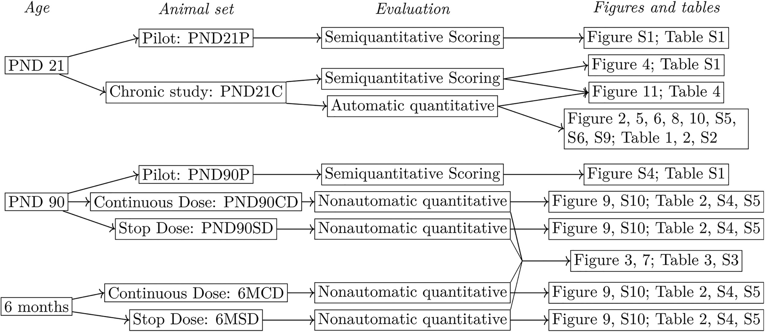
Figure 1. Study design. Each animal set contains a distinct group of animals and is therefore independent of the others. Animal groups correspond first to three different ages: PND21, PND90, and 6 months. Animals stem either from the pilot study or the main, chronic study. In the latter, animals in PND90 and 6-month groups were divided into a continuous-dose group (CD), exposed during their complete lifetime, and a stop-dose group (SD), where exposure stops at PND21. To analyze mammary glands, we used semiquantitiative scoring in PND21 and PND90. For PND21, we also used a new, automatic quantitative method. Last, for PND90 and 6-month-old animals, we used a nonautomatic quantitative method. In the subchronic (Pilot; P) study, there are animals per group per end point and the groups are Control, BPA2.5, BPA25, BPA260, BPA2700, EE2 0.5, and EE2 5.0. In the chronic study (C), animals per group per end point and the groups are Control, 2.5BPA, 25BPA, 250BPA, 2500BPA, 25000BPA, 0.05EE2, and 0.5EE2. Units: body weight (BW) per day. Note: BPA, bisphenol A; Control, vehicle control; EE2, ethinyl estradiol; PND, postnatal day.
The whole mounts were evaluated by morphometric analysis using semiquantitative methods (PND21P, PND90P, and PND21C), an automatic morphometric method (PND21C), and a standard, nonautomatic quantitative morphometric assay (PND90SD, PND90CD, 6MSD, and 6MCD). Sections of the PND90 fixed mammary glands were used to assess the time course of histoarchitectural changes and the emergence of preneoplastic and neoplastic lesions. All samples were received without knowledge of treatment group, and data were not decoded until data collection of histological and morphometric analyses were complete and the raw data were recorded in the NTP Chemical Effects in Biological Systems database.
Mammary Gland Scoring of Development
Semiquantitative mammary gland scoring.
In the subchronic BPA study (Delclos et al. 2014), the negative and positive control samples were identified a priori to the investigators and were evaluated to determine the range of response. A stereomicroscope (Nikon SMZ800; Nikon Instruments, Inc.) was used to develop the range of scores reported in Figure S1, which was modified for the range of responses in this study from the criteria reported by Davis and Fenton (2013). A score of 7 represents a gland that is most well developed, whereas a score of 1 suggests that few of the necessary developmental criteria are present. The scoring was adjusted to a 7-point scale, for both PND21 and PND90, because there was a dramatic difference between control and high-dose EE2 groups [ (Delclos et al. 2014)] in the subchronic BPA study. All whole-mounted glands were given a morphological developmental score from 1 to 7 that considered a) the number of terminal end buds (TEBs) relative to the number of duct ends, b) the degree of ductal branching and/or ductal budding, c) the number of primary ducts growing from the point of attachment, d) the degree of lobule formation, and e) the lateral and longitudinal growth of the gland (extension).
In a blinded manner, slides from PND21P-, PND21C-, and PND90P-treated and control animals were evaluated using the scoring criteria summarized in Table S1. Stacks of slides were created for each score and all mammary glands within each score were reviewed a second and third time to ensure that the scores were assigned consistently over the course of the evaluation. Two individuals with knowledge of rat mammary morphology independently evaluated all slide sets. Disagreement in score of more than a full point for any sample required reconciliation between the two scorers. When this occurred, the two scorers together revisited their scores and notes on those slides in question and decided a new score that was most appropriate given the criterion in Table S1. The new scores were less than a full point from each other.
The PND90P whole mounts were adjusted for age and stage of development. For instance, number of branch points, size, lobule formation, and density were important contributors to assigned scores.
Nonautomatic Quantitative Mammary Gland Morphometric Analysis
In the PND90 and 6-month mammary gland quantitative analysis, mammary glands from PND90P, PND90CD, PND90SD, 6MCD, and 6MSD animals were assessed for overall glandular development and density. Wet mammary gland weight was recorded at the NCTR at time of collection. The chronic study glands were imaged with a Stemi 2000 stereomicroscope (Carl Zeiss) and Axiovision software (Carl Zeiss). Image J (NIH) software ( Schneider et al. 2012) was used to process and analyze captured images to assess epithelial density of the gland (a measure of total fat pad area and epithelial area). Three standardized separate areas of each gland were measured to determine average density of the gland. Area 1 (rostral) was closer to the third mammary gland, Area 2 was in the middle of the gland, and Area 3 (caudal) was closer to the fifth mammary gland. The thickness of these whole mounts precluded a complete scan using a confocal microscope. Moreover, the thickness of these whole mounts was variable, preventing equivalent sampling. Therefore, PND90 and 6-month glands were visually scored for the following countable morphological parameters: number of leading edge/internal terminal ends, as well as incidence of lateral branching, lateral budding, alveolar budding, and lobuloalveolar development. Putative lesions identified in whole mounts were excised for histopathological assessment.
Automatic Morphometric Analysis of PND21 Mammary Glands in Chronic Study
Imaging.
In order to reduce ambiguity in the analysis due to overlapping branches, we obtained optical sections to generate a three-dimensional (3D) image instead of a bright field image of the gland. This method was only applicable to PND21 mammary glands due to their smaller size and thickness compared with the later time points. Samples were imaged with a Zeiss LSM 510 confocal microscope using the auto-fluorescence of carmine as the signal. Due to the large size of the whole glands, the imaging was done on a grid, leading to 150–600 partially overlapping stacks. The resolution used was for the optical plane (x–y) and for the depth (z). The resulting stacks were stitched in Fiji using the method described by Preibisch et al. (2009).
Identification of epithelium.
Segmentation separates a region of interest from the background. In the mammary gland, the region of interest is the epithelium, whereas the background includes the stroma and the blood and lymph vessels. Currently available algorithms for reconstructing branching structures in the vascular system (Luboz et al. 2005) cannot be used for the mammary gland owing to the presence of ductal buds (shown in Figure 2A). Therefore, we designed a custom automatic method. In addition, due to optical limitations, the presence of the lumen did not provide a consistent pattern that could be used for segmentation. Because of this limitation, we found it easier to segment the stroma first instead of focusing directly on the epithelium. The segmentation algorithm used the following steps:
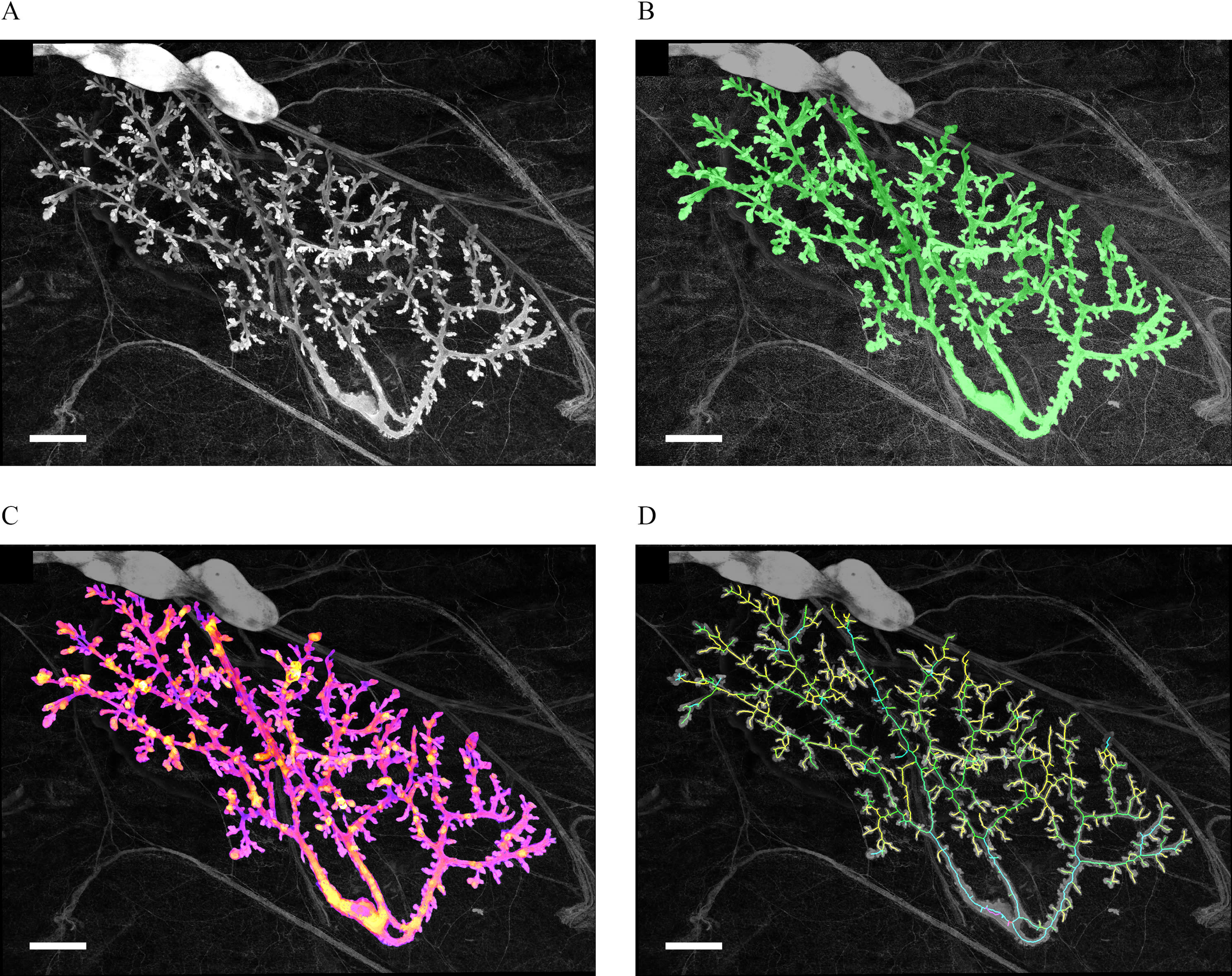
Figure 2. PND21 mammary gland from chronic study at different steps of analysis. All images are projections and all data are processed as 3D stacks. (A) Original image after stitching. (B) Green overlay of the epithelium after segmentation (identification of the epithelium). (C) Analysis of the local thickness of the epithelium, warmer colors correspond to thicker parts of the epithelium in 3D. (D) Estimated skeleton of the epithelial tree, the color of a branch corresponds to the depth of the tree that starts at this branch. Scale bars: . Note: PND, postnatal day; 3D, three-dimensional.
Step 1.
To remove nuclei of stroma cells and noise from image acquisition, we used bilateral filtering (with spatial radius 4 and range 150) followed by the subtraction of local background. The resulting image was then used for the segmentation.
Step 2.
The image was inverted, and the stroma segmented as a bright connected region, with a uniform threshold. Then, 3D Gaussian blur (radius 2) was applied to the resulting binary image to remove small structures such as blood vessels or adipocytes. Next, the image was inverted and the epithelium was obtained as the connected region above a given brightness, which included a point in the epithelial tree that had been manually selected. Holes in the epithelium, which were due to the lumen, were filled in and another Gaussian blur was performed. Finally, we performed a second selection of the connected region corresponding to the epithelium and above a given brightness. This second segmentation reduced possible artifacts that mostly stemmed from small blood vessels and adipocytes.
Step 3.
Human intervention was required for comparing the segmented epithelium with the original image. Although this means that the method is semiautomatic in the strictest sense, we will continue to refer to it as automatic here to avoid confusion. The purpose of this comparison was, first, to assess whether all the epithelium was accurately segmented. Missing epithelium typically corresponds to a loss of brightness in deeper parts of the sample or particularly thin epithelial structures. Second, the user ensured that structures other than mammary epithelium were not segmented (such as blood and lymph vessels or lymph nodes). If the output was deemed acceptable, segmentation was complete; otherwise, human intervention was required to correct the segmentation issues. Intervention corrected the stacks that were used at the beginning of Step 2. Epithelial structures lost during segmentation were recovered by increasing the brightness. Nonepithelial structures were removed either completely or by decreasing the brightness around these structures. After this operation was performed, the program went back to Step 2, performing the segmentation and subsequent verification again.
Extraction of quantitative morphological features.
The result of segmentation was a 3D reconstruction of the epithelium, which is illustrated by the green layer of Figure 2B. This representation of the epithelium was then used to extract several quantitative morphological features of mammary glands. Analyses were performed using ImageJ. Before performing these analyses, we automatically standardized the orientation of the glands on the basis of the axes of inertia. We first analyzed the properties of the 3D epithelial reconstruction on the x–y plane, which was comparable with assessments performed on bright field microscopy, such as the semiquantitative scoring. The analysis included quantities such as the aspect ratio (AR; length/width), the epithelial area, and the fractal dimension of the epithelium in two-dimensional (2D) (the projection of its 3D image). The same kind of global analysis was also performed in 3D and included an evaluation of the surface of the epithelium, of its volume, and of its 3D fractal dimension (based on the box counting method) ( Longo and Montévil 2014).
Last, the analysis used several plugins from ImageJ: the 3D object counter (Bolte and Cordelières 2006), the plugin 3D shape ( Sheets et al. 2013), and the bonej plugins (Doube et al. 2010). The latter included an evaluation of the local thickness (Figure 2C), which was performed after the normalization of the scales of the three spatial dimensions. The epithelium was skeletonized (Figure 2D) and this skeleton was analyzed by generic methods (counting the number of branches, average branch length, and so on). The analysis was performed both with and without terminal branches (pruning) given that some of the terminal branches may not have corresponded to actual epithelial structures but may have been artifacts from the process of skeletonization.
Finally, a more specialized approach to reconstructing the epithelial tree was performed by a custom plugin. This plugin started from the skeleton generated as discussed above and a manual selection of the starting point of the gland (the point of attachment). The plugin then reconstructed the mammary tree with the main duct as the root. To identify secondary branching, we performed the following operation recursively: For each branching, the size (depth) of the two subtrees was assessed; if the ratio between these depths was smaller than 0.3, then the branch associated with the smaller subtree, A, was identified as a secondary branch and the other, B, was identified as a part of the parent duct. In this case, the parent branch and B were merged. This reconstruction was then used as the basis for evaluating various properties. When quantities are defined per branch, the average over all branches is reported. To filter biologically relevant shapes, we report two versions of these quantities: one where we excluded branches smaller than and another were we excluded branches smaller than , thus removing buds. Quantities reported are, for example, the length of branches, the distance from a branch to the point of attachment counted both in terms of the number of branching points and as the sum of the lengths of the branches that linked the two. We also considered branching angles and the tortuosity of the branches (i.e., for a branch, the ratio between its length by the length of a straight line between its extremities: the less straight the branch, the higher the tortuosity). Other quantities such as the local thickness, both in 2D and 3D, were also determined by considering the average and standard deviation of their values on the skeleton points of every branch.
Overall our method assessed 91 structural features of mammary glands (see Table S2). Three complementary features were added: animal weight, mammary gland weight, and manual assessment of the number of TEBs.
Statistical Analysis
Rationale of the statistical analysis.
In the automatic analysis, six dose groups (vehicle and five BPA doses) containing 10 animals each were used and all animals came from different litters. More than 90 end points for each animal were measured to assess dose responses. This is quite different than the customary situation when one animal provides a much smaller number of end points, with the exception being certain types of -omics studies (transcriptomics-metabolomics). These situations (our quantitative measurements and the -omics) are more conducive to different types of analysis, such as principal component analysis (PCA), the permutation tests, and so on ( Goh and Wong 2018). In addition, classical statistical tests such as Dunnett’s t and Student’s t lose power rapidly when the numbers of end points and doses increase. With the number of tests necessary for our quantitative experimental designs, these tests are not generally useful.
Another consideration is that there are neither theoretical nor empirical bases that predict a specific type of dose–response curve for BPA. Empirically, BPA dose–response curves could be monotonic for some end points and nonmonotonic for other end points (Villar-Pazos et al. 2017); this is also the case with natural estrogens when comparing the effects on the uterus (monotonic) and the mammary gland (nonmonotonic), using the same animal set (Vandenberg et al. 2006). Here, we consider morphological features that are the result of nonlinear processes of morphogenesis at the tissue level in vivo, where many levels of organization are entangled.
We focus on showing that a specific dose is the locus of a breaking point that is a specific kind of nonlinear behavior and use the permutation test to assess this hypothesis. In our analysis, we distinguish exploratory and confirmatory statistics and perform both to show the presence of this breaking point. Then, we performed exploratory analysis to further characterize this response, the main biological features involved, and the shape of their response by phenomenological curve-fitting.
Principal component analysis.
We performed PCA with R (version 3.5.3; R Development Core Team) and the FactoMineR package (Lê et al. 2008). We use the dimdesc function of this package to assess the meaning of dimensions resulting from PCA and the effect of treatments; for further details see “Supplementary Analysis by PCA” in the Supplemental Material.
Global analysis to identify a breaking point.
Motivation.
In PND21C, we noted that the response curve of many features seemed to possess a specific property. However, there are several problems to analyzing this situation. a) In many cases, individual features and specific doses are not statistically significant alone because variability is high and generic corrections of multiple comparisons cripple statistical significance. b) The recurrence of this pattern could very well stem from a common, random origin because different features of an animal can be correlated. c) Introducing a specific target of statistical analysis always bears the risk of choosing a pattern specific to the data—provided that even purely random data will have patterns.
Overall strategy.
To build on the diversity of features measured above (a) and avoid errors stemming from multiple comparisons of nonindependent variables (a and b), we designed an analysis at the level of whole data sets combined. To validate the analysis beyond a single data set (c), we used the PND21C data set to formulate a precise statistical hypothesis and we used the four other animal sets of the chronic study (PND90CD, PND90SD, 6MCD, and 6MSD) together for a confirmatory analysis.
Each data set stemmed from a unique set of animals. However, the different features observed for an animal are not independent a priori (b); for example, the total length of the epithelial branches and their volume are correlated. To accommodate this complex structure, we use the permutation test. Unlike traditional tests that use a standard distribution, the permutation test builds the statistic of the intended random variable on the basis of the data and the statistical hypothesis. Because some animals of different data sets come from the same litter, we also evaluated possible litter effects by the permutation test.
Defining the random variable X.
The responses detected in PND21C were not U-shaped; instead they seem to be characterized by a sudden drop or a breaking point—these two latter patterns cannot be set apart on purely empirical bases. We used the PND21C data set to propose a variable X describing the presence of an overall breaking point between the consecutive treatments, . X is large when is the locus of the largest change for most variables over the four remaining data sets.
More precisely, for each variable measured (see list in Table S2 for PND21C), we identified the consecutive concentrations where the difference was the largest. To avoid differences that stemmed from noise, we added an algorithmic criterion to check whether a difference was large enough to be included. We proposed two types of criteria:
The first series of criteria, A( ), was met when the ratio between the mean values at consecutive conditions was larger than a threshold . The larger , the stricter this criterion became. For each variable, we looked for the consecutive concentrations with the largest ratio.
The second series of criteria, B( ), was met when a t-test between the consecutive conditions had a p-value that was smaller than a threshold . Therefore, the smaller , the stricter this criterion was. With this criterion, we compared the difference between the means of the consecutive conditions and looked for the largest difference meeting this criterion. Note, that we did not take because this condition was too strict. The aim of using the threshold was to disregard very small differences between consecutive conditions taking into account standard deviation, not to assess significance. The latter is done using the statistical test below.
We considered the variables:
Statistical hypotheses.
The null hypothesis ( ) is that the treatment did not impact the rat mammary gland morphology, or in other words that all treatment conditions are equivalent. On the basis of the PND21C data set, we formulate the alternative hypothesis [Hypothesis 1 ( )]: is higher than in , meaning that there is a remarkable change at .
Statistical test.
To assess whether our results were significant, we used the Monte Carlo permutation test (Nichols and Holmes 2002). Like most statistical tests, the permutation test assesses whether is likely under the . The statistics of X is complex because the different variables describing a mammary gland are not independent. The permutation test provides an accurate solution to this problem. The permutation test provides an estimation , of the distribution of X under the that treatment has no effect.
No effect of the treatment means that randomly shuffling the exposure group label in the data set yields an outcome that is equally probable as that of the initial data set. Therefore, performing several such permutations and computing the resulting value of X every time generates an estimation of the statistic of X: . The operation of permutation is equivalent to randomly assigning the condition (exposure) of each animal but holding the number of animals for every condition constant and, for each individual animal, preserving all its measured biological properties. Because all variables describing individual animals except their condition (BPA exposure dose) are left unchanged, all correlations between the morphological features in data sets are preserved in the permutations and taken into account in the test. The permutation test requires that the order of the observations can be exchanged. It does not require independence of the different features observed for each animal.
This operation was iterated 10,000 times to obtain the distributions of for each of our four data sets. Then we added the values of to obtain the approximate distribution of X, , under the . Because the data sets were independent, we computed by an approximation of the convolution of the distributions to obtain a more precise approximation of X. Figure 3 shows the resulting distributions for Criterion A(1.2) ( Figure 3A) and Criterion B(0.5) (Figure 3B) with . 10,000 iterations and convolutions were sufficient to obtain smooth distribution in both cases.

Figure 3. Distribution of as a result of permutations of animal exposures. X evaluates whether the change from 25BPA to 250BPA is different from changes between other consecutive concentrations in data sets from the chronic study. To evaluate the significance of results concerning X, we used the permutation test. The measurements performed in each animal were not rearranged; only the exposure labels were permutated. We computed X for 10,000 permutations and performed a convolution for the contribution of each data set. We generated the distribution , which approximates the one of X. We marked the thresholds for values higher than 95% and 99.5% of the distribution of . above this threshold leads us to decide against the with and 0.005, respectively. (A) for Criterion A(1.2) with 10,000 iterations: the ratio between consecutive values has to be at least 1.2 to be taken into account. (B) for Criterion B(0.5) with 10,000 iterations: the p-value between consecutive values has to be at least 0.5 (t-test) to be taken into account. In both cases, we see that the simulation converges toward a smooth distribution. Number of animals per group , number of groups: 6. Note: BPA, bisphenol A; , null hypothesis.
Next, we looked at the threshold ( ) for significance ( and ) in the simulated distribution . is such that 95% (0.995%) of is smaller than . Given that we did not perform multiple tests and the permutation number is high, our estimation of the p-value can be identified with the actual p-value ( Phipson and Smyth 2010). Last, we compared with to choose between the null or alternative hypothesis.
Validation.
For this method, we assessed type 1 and type 2 error rates by simulations. To this end we used distributions mimicking our data. First we used Gaussian distributions with standard deviation 1 and mean 0, a/2, a, 0, a/2, a, where a is a parameter that determines the magnitude of the breaking point (the standard deviation being 1, ). In our experimental data, we have four sets (PND90CD, PND90SD, 6MCD, 6MSD) with six doses and roughly 10 animals per group (see Figure S2). In each of our simulations, we used this format to generate data 10,000 times (1,000 times in the case of type 2 errors). To take into account correlations in our data, we also used simulations where the different Gaussian variables are correlated according to the correlations of the N first variables of the 6MCD data. For computational reasons, we estimate the statistic of X only in the first of the 10,000 generated data sets, which we expect, leads to a moderate increase of errors rates.
Mean comparisons and correlations.
The semiquantitative developmental score is a synthetic quantity where the problems mentioned above do not apply, and its use corresponds to the assumption that BPA effects are similar to EE2 effects. Analysis of variance was used to assess the effect of BPA treatment on body weight and mammary gland weight, as well as the interaction of body weight or mammary gland weight with semiquantitative developmental scores. The effect of BPA or EE2 on semiquantitative developmental scores were analyzed by Kruskal-Wallis nonparametric tests and a Dunn’s post hoc comparison of vehicle vs. treated glands [all at PND21, and at PND90 from females in the estrus stage only, and in all stages not including diestrus and metestrus (GraphPad Prism, version 7.05)]. Trends in effect were indicated at and significant effects were noted at .
For other quantitative and unsupervised measures, we used the Student’s t-test to perform an exploratory comparison of means between control, 0.5EE2 and a dose singled out by the other analyses on PND21. The normality of the distributions was assessed by the Shapiro test. When this criterion was not met, we used a simple permutation test for the absolute difference in mean. We control the false discovery rate due to multiple comparisons, q, by the location-based estimator method described in and implemented in the LBE package for R (Dalmasso et al. 2005).
We also performed multiple comparisons between control and the other doses using Dunnett’s t-test, controlling normality with the Shapiro test. To analyze correlations, we used Pearson’s product-moment correlation implemented in R (version 3.5.3; R Development Core Team). In the box plots, we define outliers using the 1.5 interquartile range method.
Regression.
To perform regression, we used the linear model (lm function of R) on variables of interest. We compared the performance of the chosen model with simpler models (having fewer parameters) with a likelihood ratio (LR) test (using the lrtest function of R). We produced graphs for the qualitative assessment of normality and the distribution of residuals in supplementary materials. Given that we were performing multiple regressions, we used the LBE package to control the false discovery rate q.
Results
We considered three hypotheses: (i) BPA effects were qualitatively similar to the effects of 0.5EE2, (ii) BPA impacted different features and/or had opposite effects of 0.5EE2, and (iii) BPA had no effect on mammary gland development.
Semiquantitative Developmental Scoring of Glands
PND21 mammary gland development.
Assessment of PND21P mammary gland development parameters showed that EE2 5.0 produced extensive ductal growth, twice the average semiquantitative developmental score of vehicle controls (see Figure S1A). These weanling mammary ductal trees displayed developmental characteristics akin to adult mammary glands (see Figure S1D). Therefore, this dose was deemed inappropriate as a positive control and doses were reduced to 0.5 and 0.05 for the chronic study. Although the effects of EE2 (at both 0.5 and 5.0) were significant, there were no statistically significant effects of BPA on the PND21P mammary glands in the subchronic study (see Figure S1A).
In the chronic study, analysis of variance did not show significant effects of BPA and EE2 exposures on the body weight of female weanlings nor on the weight of the excised mammary fat pad (see Figure S3). Scoring of PND21C mammary gland morphology revealed that only treatment with 0.5EE2 resulted in significantly different glandular development compared with vehicle control ( ) (Figure 4). There was a significant correlation between body weight and semiquantitative developmental score ( ), as well as mammary tissue weight and semiquantitative developmental score ( ). However, there was not a single dose group driving those effects (as evidenced in Figure 4).
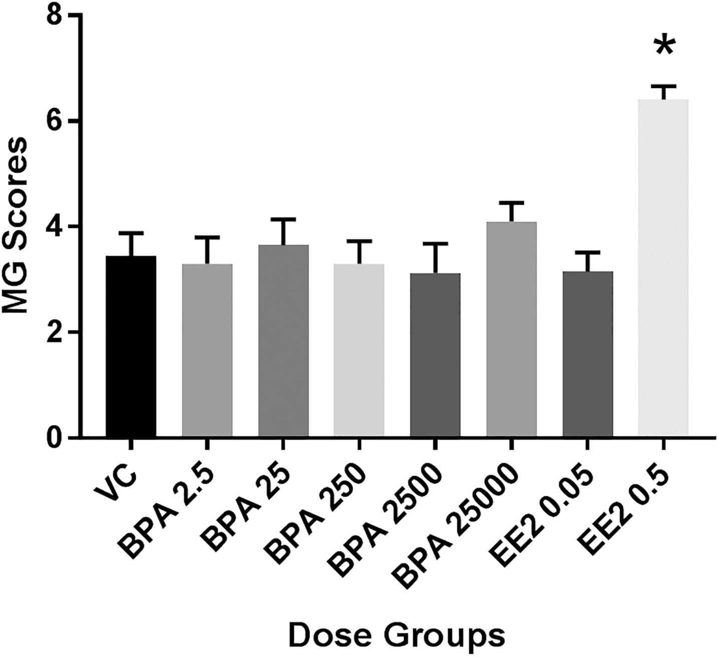
Figure 4. PND21 Mammary gland development across all exposure groups in the chronic study (Fenton group). Units: body weight (BW) per day. Based on data from the pilot 90-d subchronic study, glands were scored on a 7-point scale, where a score of 1 relates to poor development and score of 7 relates to accelerated growth and development for this age group (see Table S1). Values shown are for (2500BPA only) or 10 (all others) females per dose group. *, when compared with VC (Kruskal-Wallis, Dunn’s post hoc). Note: BPA, bisphenol A; EE2, ethinyl estradiol; MG, mammary gland; PND, postnatal day; SEM, standard error of the mean; VC, vehicle control.
PND90 and 6-month mammary gland development.
Mammary whole mounts of PND90P animals were assessed for semiquantitative developmental scoring. Females in the subchronic study were not necropsied at a predetermined stage of the estrous cycle. Analyses of semiquantitative developmental scores accounted for dose group and vaginal pathology-based cycle stage, and those data demonstrated significant estrous interaction ( ), and significantly accelerated gland development in the BPA2.5 and EE2 5.0 animals, compared with vehicle controls, when evaluated in estrus (see Figure S4A). A drop between BPA25 and BPA260, consistent with the global analysis of nonmonotonicity, was detected in animals in estrus. The EE2 0.5 and BPA25 group was also advanced in development but did not reach significance. No developmental effect of treatment (BPA or EE2) was seen when all cycle stages were considered within a group or across groups of glands (see Figure S4B).
Global Analysis: 25–250BPA as a Breaking Point
Exploratory PCA on PND21C computer-assisted morphological measurements.
PCA provided an overview of the 91 structural features (see Table S2) assessed in PN21SD mammary glands through our computational analyses, plus three additional features assessed separately (body and mammary weights and TEB number). PCA revealed that the high dose 0.5EE2 produced a strong change in mammary gland morphology (Figure 5A). Dimension (Dim) 1 represented the size of the gland and its highest correlation was with the number of branches and the surface area of the epithelium in 3D [correlation coefficient (CC): 0.97; ]. Dim 1 separated 0.5EE2 glands from the other exposure groups (t-test: ). Dim 2 was related to the thickness of ducts in 3D and was more highly correlated with the average thickness of ducts (CC: 0.84; ). Dim 2 also separated 0.5EE2-exposed glands ( , Figure 5A). Dim 3 corresponded to mean duct length (CC: 0.75; ) and separated 250BPA-exposed group from the others ( ) (Figure 5B). Dim 3 was the first dimension with significant differences for BPA exposure. Graphically, the response seemed nonmonotonic with a breaking point between 25 and 250 BPA: 2.5BPA and 25BPA are close, whereas 250BPA is very different from 25BPA and control, and high BPA doses are roughly between 25BPA and 250BPA. (Figure 5B). Dim 5 was correlated with the AR (length/width; Figure 8F presents an illustration) of the gland (0.72, ). For this variable, control was higher ( ) than the other exposure conditions. Dim 7 was correlated with the maximum duct length ( , ). For Dim 7, 25BPA was higher than other conditions ( ), whereas control and 0.5EE2 were lower ( and 0.0060, respectively).

Figure 5. Principal component analysis (PCA) of data obtained by the quantitative analysis of PND21C animals. Units: body weight (BW) per day. In all cases, we represent only the mean of each exposure group. (A) Dim 1 (correlated to the size) and Dim 2 ( ). (B) Dim 2 ( ) and Dim 3 ( ) Ellipses show some confidence intervals, and the variability of the data remains high. Number of animals per group . Note: BPA, bisphenol A; Control, vehicle control; Dim, dimension; EE2, ethinyl estradiol.
Because the dimensions of PCA depend on the data set used and EE2 conditions have a specific biological meaning, we assessed whether excluding them changes the results. We did not find a significant difference. For example, Dim 3 again separates 250BPA from other conditions ( ) (see “Supplementary analysis by PCA” in the Supplemental Material and Figure S5).
PCA provides clues against hypothesis (i), BPA effects are similar to EE2, and for (ii), BPA treatment is associated with different morphological changes than that of 0.5EE2. Moreover, PCA shows significant differences between BPA treatments and vehicle, which suggests that the hypothesis that BPA has no effect (iii) does not hold.
In the following section we assess whether the nonmonotonic pattern around 25BPA and 250BPA is real, provided that it could be nonsignificant or an artifact from PCA.
Hypothesis formulation on the basis of PND21C data sets.
We used our PND21C results as the basis to formulate our statistical hypothesis, and we used the four other independent data sets (PND90CD, PND90SD, 6MCD, 6MSD) to test this hypothesis. As detailed in the “Methods” section, a simple way to formulate our question was to look at every feature we measured and for each of them to assess which consecutive concentrations have the largest difference. We used criteria to assess differences and decide whether they were sufficient to be taken into account. With the Criterion A( ), we compared the ratio between means (met when the ratio between the consecutive conditions was larger than ), and, with Criterion B( ), we considered the arithmetic differences (met when a t-test between the consecutive conditions had a p-value smaller than the threshold ).
In PND21C, with Criterion B( ) the consecutive concentrations of 25–250BPA were associated with the largest number of changes in morphology for all values of (Table 1). Figure S6 illustrates this result graphically: yellow represents the largest difference between consecutive concentrations for a feature and the 25–250BPA column has more yellow than the others. The different criteria B( ) and A( ) provided similar results. Figure 6 illustrates the number of features having their strongest difference between each consecutive doses in the PND21C data set in comparison with data sets generated by random permutations of the treatments. The consecutive dose 25–250BPA stands out in the original data. In sets with randomly permuted doses, such an extreme situation is relatively rare but nevertheless happens occasionally when we examine all consecutive doses simultaneously. This is due to the correlations between the different variables that are preserved in permuted data (e.g., correlation between the area of a gland and its volume): Except for the treatment label, the properties of individual gland described by many variables remain unchanged in permutations. These correlations tend to increase the probability that several variables will behave in the same manner and, therefore, the frequency of large deviations (other black arrows).
Table 1 Number of observed quantities out of 94 total where the largest difference is between each consecutive condition in the PND21C data set.
| Control – 2.5BPA | 2.5 – 25BPA | 25–250BPA | 250–2500BPA | 2500BPA – 25000 BPA | |
|---|---|---|---|---|---|
| 0.05 | 3 | 0 | 17 | 0 | 0 |
| 0.5 | 14 | 5 | 57 | 6 | 9 |
| 1 (no threshold) | 15 | 6 | 52 | 7 | 9 |
Note: Differences are counted when the significance of this difference has a p-value lower than for a t-test [Criterion B( )]. BPA, bisphenol A; C, chronic study; PND, postnatal day.

Figure 6. Streamgraph of the number of quantities that have their largest difference between one of the five possible consecutive doses in PND21C. Units: body weight (BW) per day. Only differences meeting Criterion B(0.5) are taken into account. We represent the PND21C original data (left) and 20 data sets obtained by random permutations of the doses in this original data set (right of the second black vertical line). In the original data, the consecutive doses 25–250BPA is the location of the largest number of differences by far (left black arrow). In this example, situations reaching the same number of quantities than the initial data are met twice, but for another consecutive concentration (other black arrows). We use this result as a pilot to state our statistical hypotheses. : BPA exposure has no effect, and : 25–250BPA is the location of the largest change for a larger number of variables than in . Note: BPA, bisphenol A; Control, vehicle control; PND, postnatal day.
On the basis of this result and the discussion above, we hypothesized that the consecutive concentrations 25–250BPA is the locus of the largest change for most variables. For a given data set t and a given Criterion, X(t) is the proportion of quantities whose largest consecutive difference meeting the criterion is between 25BPA and 250BPA, for example, for data set PND21C and Criterion B(0.5), (based on data in Table 1). If we assume that BPA has no effect, then all five consecutive concentrations would be equivalent and we should find instead of 0.62.
We define , the sum of X(t) over all data sets (PND21C only for the exploratory analysis and all other data sets for the confirmatory analysis below; Table 2). Our statistical hypothesis is that the treatment does not impact X, and the alternative hypothesis is that is higher than under .
Table 2 Number of features for which the largest change takes place between consecutive conditions in the chronic study.
| Data set | Control to 2.5 BPA | 2.5 to 25 BPA | 25 to 250 BPA | 250 to 2 500 BPA | 2500 to 25 000 BPA | X ( t) | p-Value | |
|---|---|---|---|---|---|---|---|---|
| PND21C (training set) | 14 | 5 | 57 | 6 | 9 | 0.62 | 0.62 | 0.0094 |
| PND90CD continuous | 2 | 7 | 6 | 6 | 1 | 0.27 | 1.37 | 0.0038 |
| PND90SD | 3.5 | 3.5 | 7 | 1 | 3 | 0.39 | ||
| 6MCD | 5 | 3 | 9.5 | 0 | 6.5 | 0.40 | ||
| 6MSD | 3.5 | 8 | 7.5 | 2 | 3 | 0.31 |
Note: For Criterion B with , we find . (Table 3 reports the significance of these results.) Non-integer values stem from ties. Total number of features were 94 (PND21), 24 (PND90), and 26 (6M). BPA, bisphenol A; CD, continuous dose; M, month; PND, postnatal day; SD, stop-dose.
To assess whether we should reject in favor of , we used the permutation test on the PND21C data set. The test yields for Criterion B(0.5). This exploratory analysis suggests that we should reject for .
Confirmatory analysis with PND90CD, PND90SD, 6MCD, and 6MSD data sets.
Results.
We used the remaining, independent data sets PND90CD, PND90SD, 6MCD, and 6MSD for a confirmatory analysis. For example, Table 2 provides details in the case of Criterion B(0.5). The latter leads to and is higher than the estimated expectancy of . Note that X(t) is also higher than the estimated expectancy of 0.2 for all individual data sets. Using criteria A( ) with reasonable values of (between 1 and 1.5), we found that was significantly higher than the mean of for all significance criteria we have chosen ( ) (Table 3; Table S3). Similarly, using criteria B( ) with between 0.4 and 1, was significantly higher than the mean of ( ) with a loss of significance when the threshold was too strict or not strict enough (see Table S3). In particular, B(0.5) is the best compromise between type 1 and type 2 error rates in simulations (see Figures S2, S7, and S8) and it leads to . Figure 7 shows the contribution of each data set to the number of quantities having their largest change between each consecutive concentrations. 25–250BPA ( Figure 7A) is remarkable in comparison with the other consecutive doses (Figure 7B–E). The 20 random permutations in the figure do not reach the level of the observed data. This result illustrates the fact that the result is significant with , which is shown by more extensive simulations (Table 3; Table S3). By contrast, in Figure 7B,D,E the sum of the number of quantities in the original data sets (gray horizontal line) is below most of the permuted data. This result was expected because the consecutive concentration 25–250BPA is the locus of the largest change for many variables. Note that in Figure 7C 2.5–25BPA, this effect is not as strong.
Table 3 Comparison of and the results of the permutation test between 25 and 250BPA in PND90CD, PND90SD, 6MCD and 6MSD data sets analyzed together.
| Criterion | 95% of | 99.5% of | (litter) | ||
|---|---|---|---|---|---|
| A(1.2) | 1.67 | 1.13 | 1.38 | 0.00016 | 0.00016 |
| B(0.5) | 1.37 | 1.12 | 1.35 | 0.0038 | 0.0042 |
Note: Results for other thresholds can be found in Table S3. Criterion A(1.2) [B(0.5)] means that the ratio (p-value of a t-test, respectively) between successive means has to be at least 1.2 [0.5] to be taken into account. BPA, bisphenol A; CD, continuous dose; M, month; PND, postnatal day; SD, stop-dose.
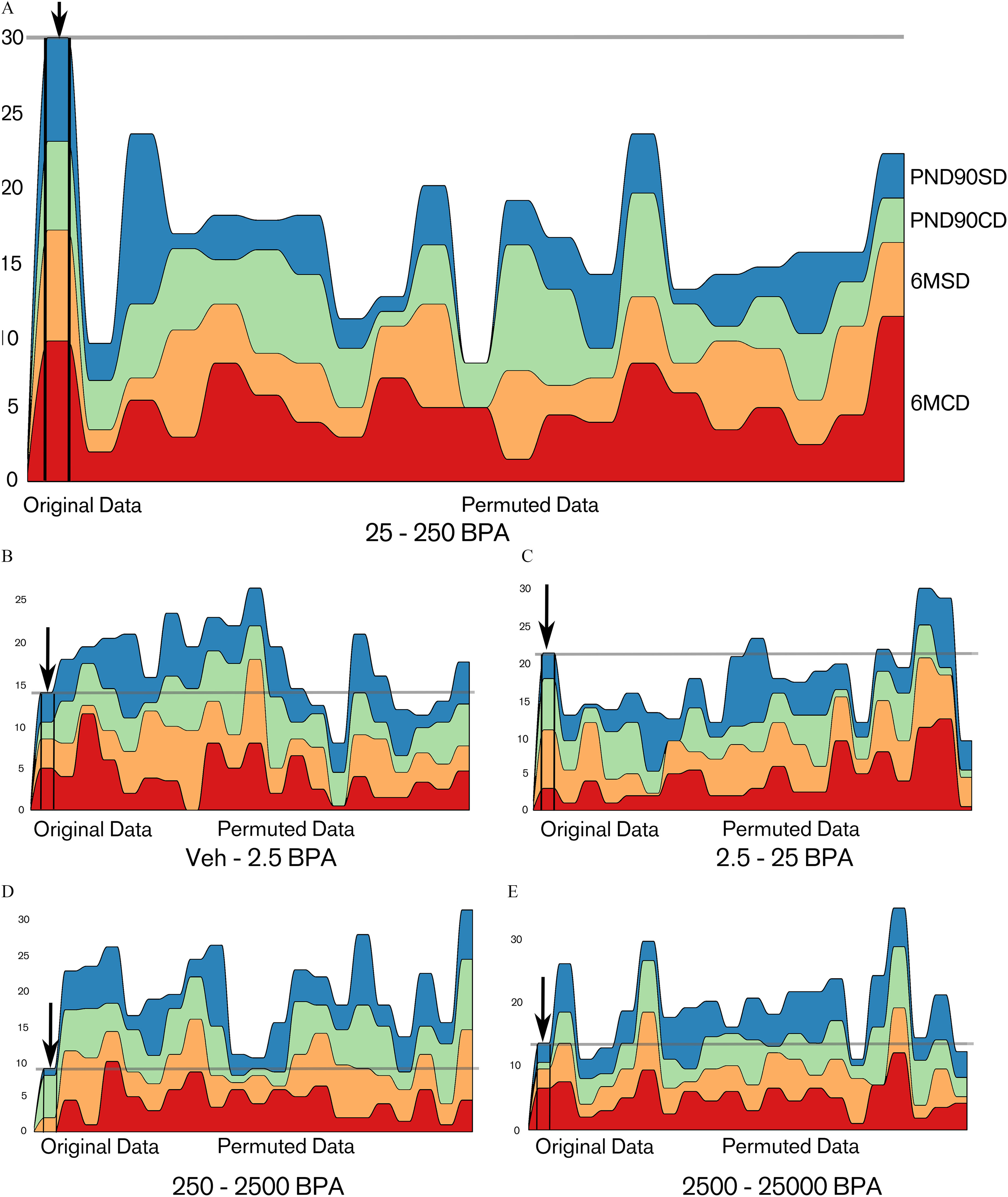
Figure 7. Number of quantities that have their largest difference between the target consecutive concentration (A) 25–250BPA and the other consecutive concentrations [(B) Veh–2.5BPA; (C) 2.5–25BPA; (D) 250–2500BPA, and (E) 2500–25000BPA] for the data sets PND90SD, PND90CD, 6MSD, and 6MCD. Units: body weight (BW) per day. In each graph: left, original data, right 20 data sets obtained by random permutation of the condition of each animal. The sum of these quantities (gray horizontal line) is higher with the original data set than with each one of the 20 permuted data sets. Note: BPA, bisphenol A; CD, continuous-dose; Control, vehicle control; M, month; PND, postnatal day; SD, stop-dose.
Taking litters into account did not change the result significantly, with . We could then safely reject the and adopt the alternative : The treatment led to a higher than if BPA did not have an effect. 25–250BPA is the locus of a jump in the dose response. A significantly high number of variables had their largest change between 25BPA and 250BPA and, accordingly, this interval was the locus of a modified response to BPA.
To conclude this global analysis, it is noteworthy that the semiquantitative scoring did, in fact, display graphically, but not robustly enough to show statistical significance, a nonmonotonic response with a slight breaking point between 25BPA and 250BPA-exposed glands in PND21C (Figure 4) and a more pronounced one in PND21P (see Figure S1) and PND90P (see Figure S4). PND21P and PND90P are animal sets that were not used in the global analysis, thus the fact that they reproduce the same pattern qualitatively is suggestive.
Validation.
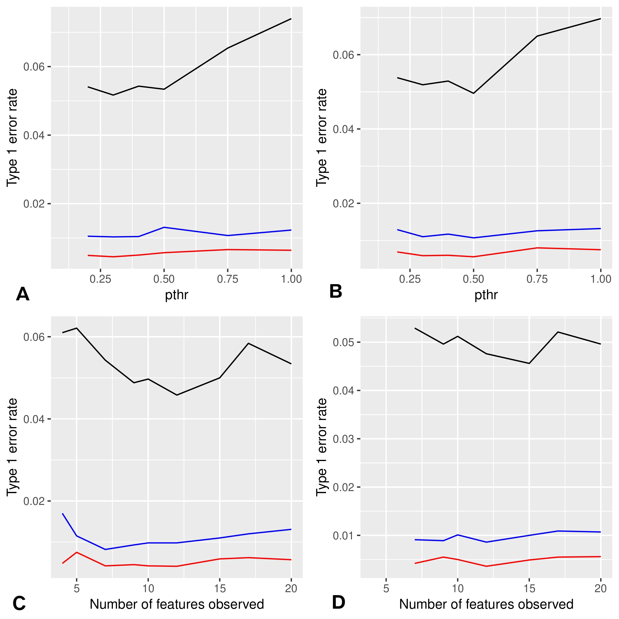
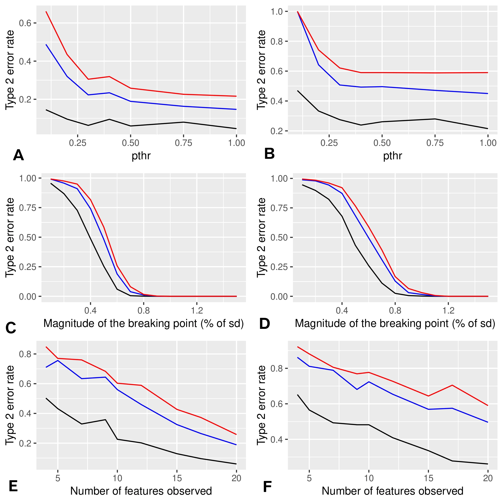
In simulations, the type 1 error rate remained close to the target with a loss of precision for or 1 (see Figure S7A). This result was consistent with the idea that those values were not restrictive enough and introduced noise in the results. The drift remained moderate and did not change in Figure S7B with correlated variables. The type 2 error rates decreased when increased (see Figure S8A,B). Overall, the type 2 error rate in simulations with correlated variables was higher, which was expected given that correlations imply a lower number of degrees of freedom (see Figure S8C,D). The higher the number of observed variables was, the lower the type 2 error rate as expected for the same reasons (see Figures S8E,F).
Further Exploratory Analysis of the Response Curve and Comparison with the Effect of EE2
PCA in PND90 and 6-month-old animals.
For PND90CD, the Dim 1 of PCA was correlated with the average density of the gland (0.88, ). For this feature, 2.5BPA was significantly higher than other conditions, whereas 250BPA was lower ( , 0.019, respectively).
For PND90SD, Dim 2 was related to the number of TEB (0.57, ) and was higher in 0.5EE2 than other conditions ( ). Dim 4 was related to epithelial area (0.75, ) and was lower in 0.5EE2 than in other conditions ( ).
For 6MCD rats, Dim 1 was related to alveolar budding (0.78, ) and for Dim 1, 0.5EE2 was lower than the other conditions ( ). Dim 4 was correlated with body weight ( , ), and 2500BPA was lower than other conditions ( ).
For 6MSD animals, Dim 1 was related to lobular alveolar budding (0.65, ). For this quantity, 0.5EE2 was higher and 250BPA was lower than the other conditions ( and 0.0018, respectively). Dim 4 was correlated with lateral budding (0.56, ) and 250BPA was lower than other conditions ( ).
Assessing nonmonotonicity.
In PND21C.
A change in the trend of the response, nonmonotonicity, was observed in various measurements obtained from PND21 mammary glands. We analyzed them with a statistical model. For example, one end point was the mean variation of ductal thickness [standard deviation (SD) width 3D], which describes whether structures are more tubular or, the opposite, irregular. This measurement is associated with budding because small buds are not recognized as individual structures and lead instead to duct width variations in the automatic analysis. This quantity increased between control and 25BPA, dropped, and then increased again between 250BPA and 25000BPA ( Figure 8A).

Figure 8. Nonmonotonic responses to BPA doses [x-axis, BPA body weight (BW) per day] shown by nonlinear regression in PND21C animals and illustration of the corresponding morphological features. Number of animals per group . Units: BW per day. The midline represents the median, the box represents the quartiles above and below the median, and the whiskers represent the two other quartiles, excluding outliers. (A–F) Graphs representing mean and standard deviation for each dose and the fit with the combination of a linear and step function. Left photomicrograph panels are representative images of a low value, right panels illustrate high values. . All features but the aspect ratio (F) show a break between 25BPA and 250BPA. In (F) the break is between 250BPA and 2500BPA. (A) Mean variation of ductal thickness: the gland on the right has many structures that have both thin and thick parts, whereas the gland on the left has more regular structures. (B) Mean thickness of the epithelium: the brightness in the pictures is proportional to the local thickness of the points of the gland. (C) Fractal dimension in 3D. The gland on the right grows more conspicuously in the third dimension than in the left figure. (D) Angle between the beginning and the end of ducts: ducts are straighter on the left and turn more on the right. (E) Third dimension from PCA. (F) AR: A large AR leads to an elongated gland, whereas a low AR means that the gland is round. Low doses of BPA increase the roundness of glands and high doses lead to an AR similar to control. Note: AR, aspect ratio; BPA, bisphenol A; Control, vehicle control; PCA, principal component analysis; PND, postnatal day; 3D, three-dimensional.
The responses detected seemed to be characterized by a sudden drop or even a breaking point, which implies two changes of trend. The model chosen for describing these data was the sum of a linear response and a step function that models a breaking point:
where a, b, and c were found by linear regression. b represents a linear trend, whereas c quantifies the sudden change between 25 and 250BPA. If b and c have opposite signs, the change between 25 and 250BPA breaks monotonicity. Note that we are not interested in the significance of a because a being different from 0 means that the average response is not 0. To assess the significance of the model, it was not sufficient to show that it fit the data significantly, we also compared it systematically with simpler models: a constant model (no effect of BPA), a linear model, and a step model. We also assessed the quality of the regression graphically (see Figure S9).
At low doses, our model described a linear response for the considered variable (0–25BPA). Then, it led to a drop in the response, which was triggered at a critical concentration that we identified by maximum likelihood. In most cases, this negative effect was between 25BPA and 250BPA. Beginning at 250BPA, increasing BPA levels resulted in a linear response. We emphasize the significance of the nonlinearity of the response that took place between 25BPA and 250BPA ( Figure 8); however, we do not make strong claims on the equational form of the model. Our model is what is usually called a phenomenological or a heuristic model; it reproduced the trends of the dose response of several end points. The choice of a specific model may only be decided by a theoretical discussion (Montévil 2018).
Given that we performed exploratory statistics on all features observed, we assessed the false discovery rate for the comparison with a constant model with the threshold . We do not report all features displaying these patterns, instead we report features with distinct biological meaning.
For SD width 3D, the nonmonotonic model led to a significant fit ( , 0.00038 for b and c, respectively). This model is significantly better than a constant model [likelihood ratio (LR) test, , ], a linear model ( ) or a step function ( ) (Figure 8A). This model captures two changes of trend because and , whereas a quadratic model can only fit one. Therefore, a quadratic model did not fit the data.
Figure 8B represents the average of the local thickness. At a point, the local thickness equals the radius of the biggest sphere that contains this point and that is contained in the structure. The model’s fit of the data was significant ( , 0.0017 for b and c, respectively), and the model was better than a constant model (LR test, and ), a linear model and a step function (LR test, , 0.019, respectively).
Figure 8C represents the fractal dimension in 3D by the box counting method. The higher this quantity, the more the epithelium had filled the fat pad of the gland in 3D. This quantity was an assessment of the complexity of the gland. The fit was significant ( , 0.011 for b and c, respectively), and the model was significantly better than a constant ( , ) and a linear model ( ), and almost better than the step model ( ). The step model alone was not a better fit ( ).
Figure 8D represents the average angle between the beginning and the end of ducts. This quantity assessed how much the ducts change direction during their growth. The fit was not entirely significant with for b and for c, and it was not significantly better than a constant model and a step model, only better than a linear model ( , 0.16 and 0.041, respectively). Nevertheless, we found this feature biologically interesting, and we will therefore discuss it again below.
Figure 8E represents the third dimension constructed by PCA, which was associated with duct length. The linear part of the model was not significant ( , 0.018 for b and c). Nevertheless it was better than a constant model and a linear model, but not a step model ( , 0.015, 0.097, respectively, ). The latter was a good fit ( ), and it was better than a constant model ( ).
Figure 8F represents the AR. This quantity equals the ratio between the largest axis of the gland and its smaller axis and was one aspect of how the epithelium invades the fat pad. For 250–2500BPA instead of 25–250BPA, our model was a good fit ( , 0.0092 for b and c, respectively), and it was better than a constant, linear, or step model ( , 0.0072, 0.027, , respectively).
The existence of various end points exhibiting a nonmonotonic response was against hypothesis (iii), which postulated that BPA is devoid of effect. The conclusion of this exploratory analysis is that nonmonotonicity can be different than quadratic (U-shaped) responses, and that features related to thickness, duct width, fractal dimension in 3D are of interest. The AR also exhibited an interesting pattern, but not with respect to the 25–250BPA breaking point.
In PND90 and 6-month.
Nonmonotonic responses in PND90CD, PND90SD, 6MCD, and 6MSD were found which were similar to the ones in PND21C (Figure 9; Figure S10). More specifically, the gland weight (determined at necropsy) in PND90SD (Figure 9A) was a significant fit to our model ( and 0.039 for b and c, respectively). The model was not significantly better than a constant model; nevertheless, the p-value is below 0.1 ( ). It was significantly better than a linear or a step model ( and 0.033, respectively).

Figure 9. Nonmonotonic mammary epithelial responses in glands from BPA-exposed PND90 and 6-month-old animals. Units: body weight (BW) per day. The midline represents the median, the box represents the quartiles above and below the median, and the whiskers represent the two other quartiles, excluding outliers. The curves represent the fit with the sum of a linear and step function and also a step model when relevant. (A) Log of mammary gland whole mount weight in PND90SD. (B–D) Density analysis in the anterior area (Area 3) in PND90CD, 6MCD, and 6MSD, respectively. In all cases, the complete model is not significant for all our statistical criteria; however, the step model is significant in B and D. Number of animals per group . Note: BPA, bisphenol A; Control, vehicle control; CD, continuous dose; M, month; PND, postnatal day; SD, stop-dose.
Interestingly, the same quantity can be described by our model in PND90CD, 6MCD, and 6MSD (Figure 9B–D). This quantity was the branching density of the posterior region of the mammary gland, closest to the fifth mammary gland (Area 3). In PN90CD, the complete model was not a good fit ( for b), but it was still better than a constant model ( , ). The step model alone was a good fit ( ) and was better than a constant model ( ).
In 6MCD, the model was a good fit ( , 0.024 for b and c, respectively), was almost significantly better than a constant model, and was better than a linear or step model ( , 0.020, 0.049, respectively, ).
In 6MSD, the situation was similar (0.11, 0.017 for b and c), was better than a constant and a linear model, and almost significantly better than a step model ( , 0.014, 0.098, respectively, ). A step model was a good fit, with ( ) and better than a constant model ( ).
Comparison between negative control, BPA inflection point, and positive control (0.5EE2).
In PND21C.
Because an inflection point was detected between 25BPA and 250BPA for several features, such as sd width 3D or the fractal dimension in 3D (Figure 8), we systematically investigated differences between 250BPA and control using the t-test for all features observed. We assessed the false discovery rate due to multiple testing with the threshold . In the cases where 250BPA was significantly different from control, we investigated whether the effect of the 0.5EE2 dose was comparable to the effect of 250BPA hypothesis (i) or was qualitatively different hypothesis (ii). Given that we investigated individual quantities, we decided against (i) and for (ii) when the effect of 0.5EE2 was lower than the one of 250BPA, which we tested by a t-test. Hypothesis (ii) can correspond to two different situations, (iia) there was no effect of 0.5EE2 by comparison with control or, alternatively, (iib) the effect of 0.5EE2 was opposite the effect of 250BPA. We used Bonferroni corrections to control multiple comparisons among treatments. Results from these comparisons are summarized and illustrated in Figure 10.

Figure 10. Comparisons between control and 250BPA, control and 0.5EE2, and 250BPA and 0.5EE2 in PND21C. (A–H) Box plots of several quantities for which the mean is significantly different between control and 250BPA. Units: body weight (BW) per day. The midline represents the median, the box represents the quartiles above and below the median, and the whiskers represent the two other quartiles, excluding outliers. p-Values correspond to t-test for control vs. 250BPA and t-test to assess whether the effect of EE2 was similar to the one of BPA, corrected for multiple comparisons. In all cases, the distributions do not differ significantly from a Gaussian distribution by the Shapiro test. Number of animals per group . (A,B) Graphs show quantities where the effects of 250BPA and 0.5EE2 are similar, matching hypothesis (i). (C–E) Graphs show quantities where 250BPA is different from Control but 0.5EE2 is not, which fits hypothesis (iia). (F–H) Graphs show features where the effects of 250BPA and 0.5EE2 are opposite, matching hypothesis (iib). (I,J) Photomicrographs show the morphological differences between Control (I) and 250BPA (J) in PND21C animals. These samples are chosen because they exhibit the differences outlined in A–H. . Note: BPA, bisphenol A; Control, vehicle control; EE2, ethinyl estradiol.
Aspect ratio.
Glands of rats exposed to 250BPA were rounder (had a smaller AR) ( , ) compared with controls. 0.5EE2 was similar to 250BPA ( ) and rounder than control ( ). The response to BPA and EE2 were similar, consistent with hypothesis (i) (Figures 8F and 10A).
Branching/budding.
The proportion of small branches (buds and small ducts ) was smaller in 250BPA than in control ( , ). For 0.5EE2, this quantity was between 250BPA and control, and closer to 250BPA (Figure 10B). This feature suggests a similar effect of BPA and EE2; compatible with hypothesis (i). The proportion of very small branches ( ) can be interpreted as epithelial budding. There was fewer very small branches in 250BPA than in the control ( , ). Against hypothesis (i), there was more very small branches in 0.5EE2 than in 250BPA group ( ). 0.5EE2 was comparable to the control (Figure 10C). This feature matches hypothesis (iia): BPA impacts a feature that EE2 does not.
Branch length measurements.
Branches were defined computationally as a path from a bifurcation to the next bifurcation. The branches were longer on average in 250BPA than in control ( , ), but their maximum length was smaller ( , ) (Figure 10D,E). Similar results were obtained when the terminal branches were removed (pruning) ( and 0.041, and 0.21, respectively). Against hypothesis (i), 0.5EE2 was different from 250BPA ( , 0.023, 0.039, and 0.032, respectively) and was similar to control for all these end points ( ). These results matched hypothesis (iia).
Angle of branches.
When removing small structures ( ), the remaining ducts tended to be straighter (turn less) in 250BPA than control ( , ). Against hypothesis (i), 250BPA ducts were also straighter than in 0.5EE2 ( ). 0.5EE2 seemed to have an opposite effect as 250BPA but it was not significant; therefore, hypothesis (ii) held, but we could not decide between (iia) and (iib) (Figures 8D and 10F).
Topological asymmetry.
The average of the number of branching points from a branch to a terminal end (average depth of subtrees) was high when the epithelial tree was more asymmetric and low when, to the contrary, it was more balanced or compact topologically. Epithelial trees were more symmetric ( , ) in 250BPA than in control. Against hypothesis (i), trees were also more symmetric in 250BPA than in 0.5EE2, ( ). Against hypothesis (iia), trees were also more symmetric in control than in 0.5EE2 ( ), Figure 10G. Here, BPA and EE2 had opposite effects, matching hypothesis (iib).
Depth of the gland.
Similarly, the overall size of the epithelium along the z-axis were lower in 250BPA than in control ( , ). The depth was also lower in 250BPA than in 0.5EE2 ( ), which invalidates hypothesis (i). Against hypothesis (iia), it was higher in 0.5EE2 than in control ( ). This feature also matches hypothesis (iib) (Figure 10H).
We also performed multiple comparisons between all treatments and control using Dunnett’s test. Despite the important loss of statistical power when performing all comparisons, we found that the average branch length was significantly longer for 2.5BPA than for control, both without ( ) and with ( ) pruning.
As illustrated in Figure 10, some of the features analyzed are consistent with hypothesis (i); the response to BPA and EE2 are similar. Others are consistent with hypothesis (ii), where BPA impacts features that EE2 does not impact (iia) and in some cases, BPA had opposite effects than EE2 (iib).
In PND90 and 6-month.
We used the same methodology as above (see Table S4). In PND90CD, the gland density was lower on average in 250BPA-exposed glands than in vehicle ( , ). 0.5EE2 was between these two conditions so that we could not decide between hypothesis (i) and (ii). Interestingly, when the three distinct gland regions (rostral, middle, and caudal) used to determine gland density were examined independently, there were treatment-dependent differences. Exposure to 0.5EE2 led to a significantly decreased gland density in the middle of the gland (Area 2) compared with vehicle ( ). Density in the rostral area (Area 1) was lower in the 250BPA group than for females dosed with either vehicle or 0.5EE2 ( , and , respectively) which is against hypothesis (i). 0.5EE2 is similar to control, which is consistent with hypothesis (iia). Lobuloalveolar budding was higher in 250BPA and 0.5EE2 than in vehicle mammary glands ( , and , respectively, permutation test), which is consistent with hypothesis (i).
Performing comparisons between control and other continuously dosed treatment groups showed that gland density (Area 2) in 25BPA and 25000BPA was lower than in vehicle controls ( and 0.0098, respectively, corrected by Dunnett’s test).
In PND90SD, lateral budding was higher in 250BPA than in vehicle, albeit not significantly ( ). In agreement with hypothesis (i), the response was similar in 0.5EE2-treated females ( ).
In 6MCD, the fat pad area was larger in 250BPA than in vehicle controls ( , ) when 0.5EE2 was not distinct from either condition. The percentage coverage was lower in 250BPA than in control and 0.5EE2 ( and , respectively), which is against hypothesis (i). The percentage coverage was higher in EE2 than control, albeit not significantly ( ), which does not decide between (iia) and (iib).
In 6MSD, the standard deviation of gland density was higher in 250BPA than in control ( , ). Comparisons with 0.5EE2 were not significant albeit the situation was closer to hypothesis (iia). In 6MSD, the percentage coverage was lower in 250BPA than in control and 0.5EE2 ( , and , respectively), which is against hypothesis (i). Lateral branching was lower in 250BPA than in control ( , permutation test, ), 0.5EE2 almost significantly lower than 250BPA and was similar to control, matching hypothesis (iia) ( permutation test). Lateral budding and alveolar budding were almost significantly lower in 250BPA than control ( , 0.054; , 0.12, respectively, permutation test) and were significantly lower in 250BPA than in 0.5EE2 ( , 0.019, respectively, permutation test). 0.5EE2 is similar to control; therefore, this result is consistent with hypothesis (iia).
Other Results
Comparison between the automatic measurements and the semiquantitative scoring of PND21C glands.
We compared the automated quantitative measurements of the glands with the semiquantitative developmental scores reported above for the chronic study and found correlations between this score and numerous morphological features. Quantities representative of the highest correlations with the score are the 2D fractal dimension of the gland (CC: 0.88, ) and the number of branches (CC: 0.86, ).
The semiquantitative developmental score was also compared with the dimensions resulting from PCA. Table 4 shows that the scoring captured aspects of the two first dimensions of PCA ( and thickness of glands, respectively) and was not correlated to Dim 3 ( ) or to any additional dimensions. This relationship between the semiquantitative developmental score and the dimensions of PCA is meaningful because it corresponds to the directionality of developmental characteristics observed between control and 0.5EE2 treated glands (Figure 11). In this sense, the semiquantitative developmental scoring criterion alone was optimized to detect effects resulting from exposure to EE2 but was not sufficient to detect significant nonlinear responses in ductal length and several other morphological features that were shown by other analyses. Nevertheless, it is important to note that semiquantitative scoring did show a nonsignificant nonmonotonic response in morphological development between 25BPA- and 250BPA-exposed glands (Figure 4; Tables S1 and S4).
Table 4 Correlation between semiquantitative scoring and the dimensions of PCA in PND21C.
| Correlation descriptors | Dim 1 ( ) | Dim 2 ( ) | Dim 3 (s) |
|---|---|---|---|
| Correlation coefficient | 0.88 | 0.023 | |
| p-Value | 0.011 | 0.84 |
Note: Dim, dimension; PCA, principal component analysis; PND, postnatal day.

Figure 11. Comparison between semiquantitative scoring and the principal components from morphological analysis in PND21C animals. Units: body weight (BW) per day. The arrow represents the semiquantitative scoring analyzed by PCA as a supplementary quantitative variable and corresponds clearly to the direction from control to 0.5EE2. The arrow’s direction does not capture the contrast between 25BPA and 250BPA, which is almost orthogonal. Number of animals per group . Note: BPA, bisphenol A; Control, vehicle control; EE2, ethinyl estradiol; PCA, principal component analysis; PND, postnatal day.
The standard deviation between the semiquantitative assessments of the two observers scoring the glands provided further insight on its relationship with the response to BPA. We interpret this standard deviation as the result of an ambiguity in evaluating the development of some glands when this development is altered. This standard deviation is negatively correlated with the proportion of small branches ( , ) and the average thickness of the gland ( , ). These features were relevant in our analysis of the nonmonotonic response of BPA, where the nonmonotonicity corresponded to a drop, consistent with a negative correlation. This suggests that the discrepancies between the assessments of the two observers were related to the nonmonotonic response to BPA and the relatively 2D evaluation of the gland on a typical microscope. BPA and EE2 resulted in different responses: EE2 accelerated gland development, whereas BPA led to abnormal development when assessed at PND21.
Histopathology in PND90 and 6-month.
Eight lesions were identified in whole mounts and histological sections from eight PND90 mammary glands across both continuous and SD-treatment groups. No lesions manifested in vehicle-treated animals and all lesions were diagnosed as benign or malignant, ranging from lobular hyperplasia, fibroadenoma, periductular fibrosis or ductal epithelial necrosis with lymphocytic infiltration to ductal carcinoma in situ (see Table S5A). Thirty-three total lesions were identified in whole mounts and excised from twenty-four 6-month mammary glands across both continuous and SD-treatment groups. Three malignant tumors (adenocarcinomas) were classified from continuous and SD 0.5EE2 treated females, and the remaining lesions/benign tumors were found in vehicle and 2.5BPA-, 25BPA-, and 25000BPA-treated females. The benign lesions included lobular or ductular alveolar dilatations (with and without secretions), periductular fibrosis (with and without lymphocytic infiltration), fibroadenomas, and adenomas (see Table S5B).
Discussion
In a rare distribution of tissues from a very large guideline-compliant study to academic grantees, we had an opportunity to evaluate mammary gland specimens from female rats from two studies on the effects of exposure to BPA and EE2. In one study animals were exposed during fetal life until weaning (PND21) while in the other exposure ended at tissue collection at PND90 and 6 months of age.
The mammary gland is considered a sensitive target for endocrine disruption. Measurable effects manifest at low levels of exposure to endocrine disruptors, and these effects appear significantly earlier than the manifestation of mammary gland cancer. Thus, there is considerable interest in including its analysis in the animal tests used for regulatory purposes (Makris 2011; Rudel et al. 2011). At present it is mentioned in a footnote in Organisation for Economic Co-operation and Development (OECD) protocols [i.e., OETC TG443, which recommends that “end points involving pup mammary glands of both sexes be included in this Test Guideline” using validated methods (OECD 2018)]. However, the animal of choice for these regulatory studies was the NCTR-derived Sprague-Dawley rat. In contrast to mouse models (Soto et al. 2013; Paulose et al. 2015), there is a paucity of reports on the effect of fetal BPA exposure on rat mammary gland morphogenesis. This is in part due to the florid structure of the ductal tree which grows more conspicuously into the third dimension and makes quantitative assessment beyond weaning challenging ( Stanko et al. 2015). This feature of the rat mammary gland hinders the use of standard morphometric tools for the analysis of the rat mammary ductal system. Instead, conventional scoring methods are used. They are called semiquantitative because they construct a score from qualitative and countable morphological features, such as terminal end buds (see Table S1). These semiquantitative methods are reproducible, fast, and reliable. In addition, because the scoring method relies on the trained human eye to interpret structures in relation to function and pathology, the scores relate to biological outcomes.
A main objective of this study was to elucidate the shape of the dose–response curve and to test three alternative hypotheses: (i) that EE2 and BPA resulted in similar qualitative effects, (ii) that BPA and EE2 affected different features or had opposite effects, and (iii) that BPA had no effect on mammary gland development. In addition, because the size and thickness of the PND21 mammary glands were compatible with confocal scanning and complete 3D reconstruction of the ductal tree, the PND21 female rats were extensively evaluated for the effects of BPA and EE2 using a quantitative new methodology specially developed for this study.
Evaluation of Early Effects in the Mammary Gland
Consistent with our long history of evaluating both rat and mouse mammary whole mounts using semiquantitative and quantitative methods, we scored and measured glands from PND21 and PND90 in these studies, blinded to treatments. In addition, we postulated that an unsupervised, quantitative, and automated method may discover effects that are difficult to ascertain using the scoring methods. We developed and describe here a method consisting of optical confocal sections to reconstruct the gland and use of appropriate algorithms for its analysis. The choice of PND21 was motivated mostly by the size of these glands and the fact that this prepubertal age precedes the florid and fast development of the ductal system due to ovarian estrogens (Cowie 1949; Masso-Welch et al. 2000; Murray et al. 2007); thus, estrogenic responses, if induced by BPA and EE2, should be detected. The hypothesis behind this choice is that the effect of BPA would be qualitatively similar to that of EE2; that is, BPA will behave as a classical estrogen. We used the same set of mammary glands to compare this new quantitative method with the standard semiquantitative method (Davis and Fenton 2013). Both the semiquantitative and the quantitative methods were able to detect significant differences between the negative control (vehicle) and the positive control (0.5EE2) (Figures 4, 5, 10; Figure S4). However, the results obtained by both methods did not support the default hypothesis used in the experimental design, that BPA and EE2 would produce the same effect on the developing mammary gland.
Evidence for a Breaking Point between 25BPA and 250BPA and Nonmonotonicity in the Dose Response
An important motivation for the development of the quantitative assay was to obtain a precise evaluation of nonmonotonicity. There are inherent differences in assumptions about the shape of the dose–response curve in endocrinology and toxicology. The default assumption in toxicology is monotonicity. In contrast, nonmonotonic dose–response curves are a common occurrence in endocrinology. For instance, the proliferative response for estrogens and androgens follows inverted-U patterns (Stormshak et al. 1976; Amara and Dannies 1983; Soto et al. 1995; Maffini et al. 2002; Geck et al. 2000) and the effect of estradiol on the growth of the mammary ductal system is also nonmonotonic ( Vandenberg et al. 2006). Moreover, distinct end points show different estrogen dose–response curves in different organs of the same animal set: The uterotrophic assay and various other uterine morphological end points are clearly monotonic, whereas those pertaining to ductal mammary gland morphogenesis show mostly nonmonotonic dose–response curves ( Vandenberg et al. 2006).
As expected from examples in the literature, the BPA dose–response showed evidence for nonmonotonicity on data from the quantitative method in PND21C ( Jenkins et al. 2011; Cabaton et al. 2011). The dose–response curves observed for several features was not that of an inverted-U shape, instead it seemed to be characterized by a sudden drop or a breaking point located between 25BPA and 250BPA ( Jenkins et al. 2011).
We used the 91 distinct measurements obtained with the automated method for the analysis of PND21C glands to formulate a statistical test to assess whether 25–250BPA was the locus of a breaking point for a significant number of features. In this data set, our exploratory analysis by the permutation test led us to reject the hypothesis that BPA has no effect in favor of the existence of a breaking point between 25BPA and 250BPA ( Figure 6). To confirm this exploratory result, we used the smaller number of quantitative end points measured at PND90 and 6 months of age. This breaking point in the dose–response to BPA was confirmed by a single, global statistical analysis using the same permutation test (Figure 7). The key of this global analysis is the hypothesis that the breaking point between 25BPA and 250BPA is present at all time points. Again, the test leads us to reject the hypothesis that BPA has no effect in favor of a breaking point between 25BPA and 250BPA. We want to emphasize that performing this single test as a confirmatory analysis, when PND21C is used for the exploratory analysis, is a very rigorous analysis because it avoids making multiple comparisons for the many features and several data sets available. Moreover, the permutation test rigorously accommodates the individuality of each animal (i.e., the test takes into account that many features are correlated). Our overall strategy has been to build on the nonlinear feature observed in PND21C, the breaking point, in order to provide evidence that it remains valid in the other data sets taken together. Although there were no significant discernible effects in the subchronic PND21P mammary glands across BPA-treated groups, the reduced gland development in BPA260 compared with BPA25-exposed animals is consistent with the global analysis obtained from the chronic study animals (PND21C). In addition, in the 90-d subchronic pilot studies (see Figures S1 and S4), the increased development scores in the lowest BPA dose groups is another confirmation of this rationale, even though it failed to reach significance.
Once we have concluded that 25–250BPA is a breaking point, we could perform an exploratory analysis of which features are involved and the more specific shape of the dose response. Here, the analysis is performed with data sets already taken into account above; therefore, it cannot provide a confirmation of the presence of the breaking point. However, it is useful to assess the overall response curve and the features that best represent it. The model chosen was the sum of a linear response and step function because it is significantly better than either a linear model or a step function alone (Figure 8). In PND21C, for many variables, our model appears as a linear response at low doses; a drop in the response appears between 25BPA and 250BPA for most relevant features. At higher BPA doses, a linear response is observed again ( Figure 8). The most striking feature of the dose–response curve is the nonlinearity of the response that takes place between the 25BPA and 250BPA dose. In other data sets, specific quantities were also nonmonotonic such as gland weight in PND90SD and branching density in PND90CD, 6MCD, and 6MSD (Figure 9). Moreover, pair-wise and comparisons between 250BPA, 0.5EE2, and control revealed that some features are consistent with hypothesis (i), namely, the effects of EE2 and BPA are similar, and others with hypothesis (ii), namely, they are different, sometimes opposite ( Figure 10).
These results show the importance of establishing and using statistical methods appropriate for nonmonotonic responses. Linear models are a powerful tool to provide evidence of a causal relationship because they quantitatively relate the changes of a putative cause with the one of the effects. Moreover, linear responses to small causes are a common mathematical property albeit not universal. Therefore, exhibiting a linear response is a powerful method to provide empirical evidence of a causal relationship in a given context. However, this method is blind to nonmonotonic responses. The latter are common in endocrinology because the putative causes are involved in multilevel, complex regulations due to the evolutionary history of hormones and their functions. In this context, a more appropriate way to show the presence of causation is to show the prevalence of a specific nonmonotonic pattern, here a breaking point between 25BPA and 250BPA.
Semiquantitative Scoring and Quantitative Analyses
In PND21C, the scoring method captured the directionality of development as the arrow linking controls with 0.5EE2-treated (Figure 11) in the first two dimensions of PCA of data obtained by the quantitative method (correlated respectively with size and thickness). Indeed, the fact that the scoring method uses EE2 as the control implies that it would preferentially capture the effects of BPA when they mimic those of natural estrogens. Many of the features measured by the quantitative method do not relate directly to the features used for the scoring method, but still provide information about them. For example, the fractal dimension assesses the complexity of the ductal system and the mean variation of ductal thickness is associated with budding. Several of these unique features revealing significant BPA effects when evaluated in 3D are illustrated in Figure 8.
In PND21C, the data and analysis presented here demonstrate that the quantitative method, by using a multitude of automatic measurements, resulted in a greater sensitivity than the semiquantitative method to discriminate effect differences due to BPA dose. The difference between the methods reside in the fact that the quantitative method does not depend on a positive control to score development, and thus is blind to whether the effect of BPA is similar or not to that of EE2 and that the quantitative method interrogates effects existing in the third dimension (i.e., thickness, fractal dimension in 3D, angles).
In PND90 and 6-month-old animals, the scoring method revealed a significant effect of BPA in PND90P mammary glands exposed to BPA from gestation to tissue harvest. This effect was observed only at the BPA2.5 dose and only when the animals were humanely euthanized at estrus, a result consistent with the nonmonotonicity observed at all time points using the quantitative methods. The stage of the estrous cycle by itself appeared to affect the morphological outcomes, thereby validating the importance of assessing all the tissues at the same stage of the cycle for the determination of treatment effect. In fact, the effect of EE20.5 on an increased semiquantitative developmental score was not evident when glands from animals in all stages of the estrous cycle were considered (see Figure S4B). Moreover, these data also suggest that unlike the results in prepuberal PND21 animals, BPA may act in conjunction with endogenous estrogens in adult animals and thus produce a more estrogen-like pattern than that observed for BPA at PND21, that is, consistent with hypothesis (i).
The data presented here demonstrate that PND90 is an appropriate time point to assess the effect of low BPA doses and to reveal nonmonotonicity. They also highlight the importance of assessing the tissue at the same stage in the estrous cycle given that even the pronounced proliferative effect of the positive control on mammary epithelium was not evident when estrous stage was not taken into account in the data analyses. Our results also suggest that EE2 is not a good control for mammary gland end points because the effects of BPA and EE2 were distinct and there was no effect of the 0.05EE2, as expected; leaving us to suppose that the NCTR rat strain may be particularly estrogen insensitive. In summary, most of the results in these sets of mammary glands from cycling rats are consistent with hypothesis (ii), and inconsistent with hypothesis (iii).
Cancer: This Study and the Core Study
As in the mouse model, some effects of BPA are not similar to those of estrogens, for example, inhibition of ductal growth at puberty (Markey et al. 2001; Muñoz-de-Toro et al. 2005), enhanced ductal growth during fetal life ( Vandenberg et al. 2007; Speroni et al. 2017), others are clearly estrogen-like, such as the increased score at PND90P reported here and the accelerated expression of lateral branching in the mouse ( Muñoz-de-Toro et al. 2005). There are also other effects seemingly unrelated to estrogenicity; changes in the stromal fraction of the gland and inflammatory cell responses that have been noted in response to developmental BPA exposures (Tucker et al. 2018; Wadia et al. 2013).
Given that BPA is rapidly metabolized and does not bioaccumulate, the increased propensity of developing mammary cancer in animals exposed to BPA during organogenesis has been attributed to its direct effect on fetal mammary gland development and its indirect effects through the developing hypothalamic–pituitary–ovarian axis (HPOA) (Soto et al. 2013). In the present study, both PND90 and 6-month SD animals displayed a nonmonotonic response to BPA, which confirms the long-lasting effects of early BPA exposure (Table 2). The direct effect of BPA on fetal mammary gland development has been verified using fetal mammary gland explants in an ex vivo model (Speroni et al. 2017). Fetal exposure to BPA affects all the organs of the HPOA, altering ovarian steroidogenesis (Mahalingam et al. 2017; Peretz et al. 2011), hypothalamic controls of luteinizing hormone levels ( Rubin et al. 2006; Acevedo et al. 2018), and the gonadotroph number in the fetal pituitary (Brannick et al. 2012). These alterations, in turn, suggest altered regulation of mammotropic hormones ( Soto et al. 2013). Consistent with these findings, fetal exposure to BPA in mice not only affected the fetal period of mammary gland organogenesis, but also postnatal development, long after cessation of exposure. Alterations in ductal elongation at puberty and lateral branching and budding during adulthood were attributed to altered responses to mammotropic hormones such as estradiol and progesterone (Wadia et al. 2007; Ayyanan et al. 2011). Recent studies confirmed that developmental exposures to other BPA-related substances (Bisphenol S and Bisphenol AF) in mice also induce precocious development of the mammary epithelium and increased epithelial lesions and mammary tumors in adulthood (Tucker et al. 2018). However, these results were obtained in the mouse, which is not considered as good a model for mammary cancer as the rat. In spite of this widely held opinion, developmental exposure to BPA in mice also increased the incidence of mammary cancer in animals treated with a chemical carcinogen during adulthood or in MMTV-erbB2 mice exposed to BPA during adulthood ( Jenkins et al. 2011). It is remarkable that in this model, the effect of BPA was nonmonotonic. Several studies using different rat strains reported the development of hyperplasia, carcinoma in situ and palpable adenocarcinomas of the mammary gland after prenatal or neonatal exposure to BPA ( Mandrup et al. 2016; Murray et al. 2007). Not surprisingly, the CLARITY core study, run concurrently to this study, revealed a significant increase of adenocarcinomas as well as the combination of adenomas or adenocarcinomas in the SD animals treated with 2.5BPA at 2 years of age. EE2 induced a significant increase of adenocarcinomas only at the high dose and they were also detected in our animals (see Table S5) by 6 months of age.
Conclusions
Here we demonstrated that semiquantitative and quantitative methods were suitable to detect estrogenic effects in the mammary glands of NCTR SD rats, and both methods found BPA-induced mammary effects to be different from those of EE2. In addition, the semiquantitative method, by relying on the trained human eye, is better able to interpret structures in relation to function and pathology. The automatic quantitative method, by using a multitude of measurements in 3D, identified statistically significant differences and revealed a nonmonotonic BPA dose–response curve in mammary samples from PND21 animals. The nonmonotonic response was confirmed by a global analysis of quantitative assessment in mammary samples from older animals within the same study. These results show that we can and should take advantage of nonmonotonic properties to perform statistical analysis rigorously, and that these features are not limited to quadratic responses.
Consistent with our finding, the CLARITY core study, which used animals of the same cohort, found that EE2 and BPA are not similar. In the core study EE2 increased the incidence of neoplastic lesions only at the highest dose, whereas BPA only increased their incidence at the lowest dose. The BPA effect was nonmonotonic and differed between the SD and the continuous exposure regime. Thus, dose and duration of exposure contribute to the developmental and neoplastic outcomes. These data are consistent with the multiple non-GLP studies previously conducted demonstrating low-dose BPA exposures induce more adverse responses than high doses and that some low-dose BPA responses are different from those of estrogens and of high-dose BPA.
Acknowledgments
We acknowledge the technical help provided by L. Camacho and B. Delclos regarding the generation of animals and the dissection of the mammary glands examined in this study. We are also grateful to B. Davis for the histological assessment of the lesions and to our colleagues at Tufts University, C. Sonnenschein and B. Rubin, for their critical reading of the manuscript. We thank S. Baker (National Cancer Institute) for useful suggestions about the statistical design of this study. We are grateful to M. Tremblay-Franco (section of Statistics and Bioinformatics, Plateform MetaToul-AXIOM, INRA Toulouse) and K. Shockley [National Institute of Environmental Health Sciences (NIEHS)] for their critical reading and useful suggestions regarding statistical analysis. This work was supported by grant U01ES020888 from the NIEHS (A.M.S.) and NIEHS funding 1Z01ES102785 (S.E.F. and M.B.). The content is solely the responsibility of the authors and does not necessarily represent the official views of the NIEHS or the National Institutes of Health.
References
Acevedo N, Davis B, Schaeberle CM, Sonnenschein C, Soto AM . 2013. Perinatally administered bisphenol A as a potential mammary gland carcinogen in rats. Environ Health Perspect 121(9):1040–1046, PMID:23876597 , doi: 10.1289/ehp.1306734., Google ScholarAcevedo N, Rubin BS, Schaeberle CM, Soto AM . 2018. Perinatal BPA exposure and reproductive axis function in CD-1 mice. Reprod Toxicol 79:39–46, PMID:29752986 , doi: 10.1016/j.reprotox.2018.05.002. , Google ScholarAmara JF, Dannies PS . 1983. 17β-Estradiol has a biphasic effect on GH cell growth. Endocrinology 112(3):1141–1143, PMID:6822206 , doi: 10.1210/endo-112-3-1141. , Google ScholarAmrhein V, Greenland S, McShane B . 2019. Scientists rise up against statistical significance. Nature 567(7748):305–507, PMID:30894741 , doi: 10.1038/d41586-019-00857-9. , Google ScholarAyyanan A, Laribi O, Schuepbach-Mallepell S, Schrick C, Gutierrez M, Tanos T, 2011. Perinatal exposure to bisphenol A increases adult mammary gland progesterone response and cell number. Mol Endocrinol 25(11):1915–1923, PMID:21903720 , doi: 10.1210/me.2011-1129. , Google ScholarBolte S, Cordelières FP . 2006. A guided tour into subcellular colocalization analysis in light microscopy. J Microsc 224(Pt 3):213–232, PMID:17210054 , doi: 10.1111/j.1365-2818.2006.01706.x. , Google ScholarBrannick KE, Craig ZR, Himes AD, Peretz JR, Wang W, Flaws JA, 2012. Prenatal exposure to low doses of bisphenol A increases pituitary proliferation and gonadotroph number in female mice offspring at birth. Biol Reprod 87(4):82, PMID:22875908 , doi: 10.1095/biolreprod.112.100636. , Google ScholarCabaton NJ, Canlet C, Wadia PR, Tremblay-Franco M, Gautier R, Molina J, 2013. Effects of low doses of bisphenol A on the metabolome of perinatally exposed CD-1 mice. Environ Health Perspect 121(5):586–593, PMID:23425943 , doi: 10.1289/ehp.1205588. Link, Google ScholarCabaton NJ, Wadia PR, Rubin BS, Zalko D, Schaeberle CM, Askenase MH, 2011. Perinatal exposure to environmentally relevant levels of bisphenol A decreases fertility and fecundity in CD-1 mice. Environ Health Perspect 119(4):547–552, PMID:21126938 , doi: 10.1289/ehp.1002559. Link, Google ScholarCalafat AM, Kuklenyik Z, Reidy JA, Caudill SP, Ekong J, Needham JL . 2005. Urinary concentrations of bisphenol A and 4-nonylphenol in a human reference population. Environ Health Perspect 113(4):391–395, PMID:15811827 , doi: 10.1289/ehp.7534. Link, Google ScholarChristiansen S, Hass U . 2015. Evaluation of EFSA’s new Scientific Opinion on Bisphenol A. https://orbit.dtu.dk/en/publications/evaluation-of-efsas-new-scientific-opinion-on-bisphenol-a [accessed13 April 2020 ].Google ScholarChurchwell MI, Camacho L, Vanlandingham MM, Twaddle NC, Sepehr E, Delclos KB, 2014. Comparison of life-stage-dependent internal dosimetry for bisphenol A, ethinyl estradiol, a reference estrogen, and endogenous estradiol to test an estrogenic mode of action in Sprague Dawley rats . Toxicol Sci 139(1):4–20, PMID:24496641 , doi: 10.1093/toxsci/kfu021. , Google ScholarCohn BA, La Merrill M, Krigbaum NY, Yeh G, Park JS, Zimmermann L, 2015. DDT exposure in utero and breast cancer. J Clin Endocrinol Metab 100(8):2865–2872, PMID:26079774 , doi: 10.1210/jc.2015-1841. , Google ScholarCowie AT . 1949. The relative growth of the mammary gland in normal gonadectomized and adrenalectomized rats. J Endocrinol 6(2):145–147, PMID:15392907 , doi: 10.1677/joe.0.0060145. , Google ScholarDalmasso C, Broët P, Moreau T . 2005. A simple procedure for estimating the false discovery rate. Bioinformatics 21(5):660–668, PMID:15479710 , doi: 10.1093/bioinformatics/bti063. , Google Scholar- Davis B, Fenton S.2013. The mammary gland. In:
Haschek and Rousseaux’s Handbook of Toxicologic Pathology, vol. 3. 3rd ed.
Haschek WM, Rousseaux CG, Wallig MA, Ochoa R, Bolon B , eds. New York, NY: Elsevier, 2665–2694., Google Scholar Delclos KB, Camacho L, Lewis SM, Vanlandingham MM, Latendresse JR, Olson GR, 2014. Toxicity evaluation of bisphenol A administered by gavage to Sprague Dawley rats from gestation day 6 through postnatal day 90. Toxicol Sci 139(1):174–197, PMID:24496637 , doi: 10.1093/toxsci/kfu022. , Google ScholarDiamanti-Kandarakis E, Bourguignon JP, Giudice LC, Hauser R, Prins GS, Soto AM, 2009. Endocrine-disrupting chemicals: an Endocrine Society scientific statement. Endocr Rev 30(4):293–342, PMID:19502515 , doi: 10.1210/er.2009-0002. , Google ScholarDoerge DR, Vanlandingham M, Twaddle NC, Delclos KB . 2010. Lactational transfer of bisphenol A in Sprague–Dawley rats. Toxicol Lett 199(3):372–376, PMID:20933065 , doi: 10.1016/j.toxlet.2010.09.022. , Google ScholarDoube M, Kłosowski MM, Arganda-Carreras I, Cordelières FP, Dougherty RP, Jackson JS, 2010. BoneJ: free and extensible bone image analysis in ImageJ. Bone 47(6):1076–1079, PMID:20817052 , doi: 10.1016/j.bone.2010.08.023. , Google ScholarDurando M, Kass L, Piva J, Sonnenschein C, Soto AM, Luque EH, 2007. Prenatal bisphenol A exposure induces preneoplastic lesions in the mammary gland in Wistar rats. Environ Health Perspect 115(1):80–86, PMID:17366824 , doi: 10.1289/ehp.9282. Link, Google Scholar- ECHA (European Chemicals Agency). 2017.
European Chemicals Agency Support Document for Identification of 4,4′-Isopropyldenediphenol (Bisphenol A, BPA) as a substance of very high concern because of its endocrine disrupting properties (Article 57(F)) causing
probable serious effects to the environment which gives rise to an Equivalent level of concern to those of CMR1 AND PBT/vPvB2 properties
.
https://echa.europa.eu/documents/10162/13638/svhc_msc_support_document_bisphenol_a_en.pdf
[accessed
13 April 2020 ].Google Scholar - ECHA. 2020. Bisphenol A.
https://echa.europa.eu/hot-topics/bisphenol-a [accessed
13 April 2020 ].Google Scholar Geck P, Maffini MV, Szelei J, Sonnenschein C, Soto AM . 2000. Androgen-induced proliferative quiescence in prostate cancer: the role of AS3 as its mediator. Proc Natl Acad Sci USA 97(18):10185–10190, PMID:10963680 , doi: 10.1073/pnas.97.18.10185. , Google ScholarGerona RR, Woodruff TJ, Dickenson CA, Pan J, Schwartz JM, Sen S, 2013. Bisphenol-A (BPA), BPA glucuronide, and BPA sulfate in midgestation umbilical cord serum in a northern and central California population. Environ Sci Technol 47(21):12477–12485, PMID:23941471 , doi: 10.1021/es402764d. , Google ScholarGoh WWB, Wong L . 2018. Dealing with confounders in omics analysis. Trends Biotechnol 36(5):488–498, PMID:29475622 , doi: 10.1016/j.tibtech.2018.01.013. , Google ScholarHass U, Christiansen S, Boberg J, Rasmussen MG, Mandrup K, Axelstad M . 2016. Low-dose effect of developmental bisphenol A exposure on sperm count and behaviour in rats. Andrology 4(4):594–607, PMID:27089241 , doi: 10.1111/andr.12176. , Google ScholarHehn RS . 2016. NHANES data support link between handling of thermal paper receipts and increased urinary bisphenol A excretion. Environ Sci Technol 50(1):397–404, PMID:26583963 , doi: 10.1021/acs.est.5b04059. , Google ScholarHeindel JJ, Newbold RR, Bucher JR, Camacho L, Delclos KB, Lewis SM, 2015. NIEHS/FDA CLARITY-BPA research program update. Reprod Toxicol 58:33–44, PMID:26232693 , doi: 10.1016/j.reprotox.2015.07.075. , Google ScholarHoover RN, Hyer M, Pfeiffer RM, Adam E, Bond B, Cheville AL, 2011. Adverse health outcomes in women exposed in utero to diethylstilbestrol. N Engl J Med 365(14):1304–1314, PMID:21991952 , doi: 10.1056/NEJMoa1013961. , Google Scholar- IBCERCC (Interagency Breast Cancer and the Environment Research Coordinating Committee). 2013.
Breast Cancer and the Environment: Prioritizing Prevention.
http://www.niehs.nih.gov/about/assets/docs/ibcercc_full_508.pdf [accessed
13 April 2020 ].Google Scholar - INERIS (French National Institute for Industrial Environment and Risks). 2015.
Implementation of legislation regulating BPA in food-contact materials.
https://substitution-bp.ineris.fr/en/news/france-january-1st-2015-legal-text-no-2012-1442-december-24-2012
[accessed
20 April 2020 ].Google Scholar Jenkins S, Wang J, Eltoum I, Desmond R, Lamartiniere CA . 2011. Chronic oral exposure to bisphenol A results in a nonmonotonic dose response in mammary carcinogenesis and metastasis in MMTV-erbB2 mice. Environ Health Perspect 119(11):1604–1609, PMID:21988766 , doi: 10.1289/ehp.1103850. Link, Google ScholarKotsopoulos J, Chen WY, Gates MA, Tworoger SS, Hankinson SE, Rosner BA . 2010. Risk factors for ductal and lobular breast cancer: results from the Nurses’ Health Study. Breast Cancer Res 12(6):R106, PMID:21143857 , doi: 10.1186/bcr2790. , Google ScholarLamartiniere CA, Jenkins S, Betancourt AM, Wang J, Russo J . 2011. Exposure to the endocrine disruptor bisphenol A alters susceptibility for mammary cancer. Horm Mol Biol Clin Investig 5(2):45–52, PMID:21687816 , doi: 10.1515/HMBCI.2010.075. , Google ScholarLê S, Josse J, Husson F . 2008. FactoMineR: an R package for multivariate analysis. J Stat Softw 25(1):1–18, doi: 10.18637/jss.v025.i01., Google ScholarLewis SM, Lee FW, Ali AA, Allaben WT, Weis CC, Leakey JE . 2010. Modifying a displacement pump for oral gavage dosing of solution and suspension preparations to adult and neonatal mice. Lab Anim (NY) 39(5):149–154, PMID:20410899 , doi: 10.1038/laban0510-149. , Google ScholarLongo G, Montévil M . 2014. Perspectives on Organisms: Biological Time, Symmetries and Singularities. Berlin, Germany: Springer, doi: 10.1007/978-3-642-35938-5., Google ScholarLuboz V, Wu X, Krissian K, Westin C-F, Kikinis R, Cotin S . 2005. A segmentation and reconstruction technique for 3D vascular structures, In: Proceedings of the Medical Image Computing and Computer-Assisted Intervention—MICCAI 2005: 8th International Conference, Palm Springs, CA, 26–29 October, 2005, Part I, Berlin, Germany: Springer, 43–50, doi: 10.1007/11566465_6., Google ScholarMaffini MV, Calabro JM, Soto AM, Sonnenschein C . 2005. Stromal regulation of neoplastic development: age-dependent normalization of neoplastic mammary cells by mammary stroma. Am J Pathol 167(5):1405–1410, PMID:16251424 , doi: 10.1016/S0002-9440(10)61227-8. , Google ScholarMaffini MV, Geck P, Powell CE, Sonnenschein C, Soto AM . 2002. Mechanism of androgen action on cell proliferation AS3 protein as a mediator of proliferative arrest in the rat prostate. Endocrinology 143(7):2708–2714, PMID:12072405 , doi: 10.1210/endo.143.7.8899. , Google ScholarMahalingam S, Ther L, Gao L, Wang W, Ziv-Gal A, Flaws JA . 2017. The effects of in utero bisphenol A exposure on ovarian follicle numbers and steroidogenesis in the F1 and F2 generations of mice. Reprod Toxicol 74:150–157, PMID:28970132 , doi: 10.1016/j.reprotox.2017.09.013. , Google ScholarMakris SL . 2011. Current assessment of the effects of environmental chemicals on the mammary gland in guideline rodent studies by the U.S. Environmental Protection Agency (U.S. EPA), Organisation for Economic Co-operation and Development (OECD), and National Toxicology Program (NTP) . Environ Health Perspect 119(8):1047–1052, PMID:21118785 , doi: 10.1289/ehp.1002676. Link, Google ScholarMandrup K, Boberg J, Isling LK, Christiansen S, Hass U . 2016. Low-dose effects of bisphenol A on mammary gland development in rats. Andrology 4(4):673–683, PMID:27088260 , doi: 10.1111/andr.12193. , Google ScholarMarkey CM, Luque EH, Munoz de Toro MM, Sonnenschein C, Soto AM . 2001. In utero exposure to bisphenol A alters the development and tissue organization of the mouse mammary gland. Biol Reprod 65(4):1215–1223, PMID:11566746 , doi: 10.1093/biolreprod/65.4.1215. , Google ScholarMasso-Welch PA, Darcy KM, Stangle-Castor NC, Ip MM . 2000. A developmental atlas of rat mammary gland histology. J Mammary Gland Biol Neoplasia 5(2):165–185, PMID:11149571 , doi: 10.1023/a:1026491221687. , Google Scholar- Montévil M.2018. A primer on mathematical modeling in the study of organisms and their parts. In:
Systems Biology. Methods in Molecular Biology.
Bizzarri M , ed. New York, NY: Humana Press, 41–55, doi: 10.1007/978-1-4939-7456-6_4., Google Scholar Montévil M . 2019. Measurement in biology is methodized by theory. Biol Philos 34:35, doi: 10.1007/s10539-019-9687-x., Google ScholarMuñoz-de-Toro MM, Markey CM, Wadia PR, Luque EH, Rubin BS, Sonnenschein C, 2005. Perinatal exposure to bisphenol A alters peripubertal mammary gland development in mice. Endocrinology 146(9):4138–4147, PMID:15919749 , doi: 10.1210/en.2005-0340. , Google ScholarMurray TJ, Maffini MV, Ucci AA, Sonnenschein C, Soto AM . 2007. Induction of mammary gland ductal hyperplasias and carcinoma in situ following fetal bisphenol A exposure. Reprod Toxicol 23(3):383–390, PMID:17123778 , doi: 10.1016/j.reprotox.2006.10.002. , Google ScholarNichols TE, Holmes AP . 2002. Nonparametric permutation tests for functional neuroimaging: a primer with examples. Hum Brain Mapp 15(1):1–25, PMID:11747097 , doi: 10.1002/hbm.1058. , Google Scholar- OECD (Organisation for Economic Co-operation and Development). 2018.
Test No. 443: Extended One-Generation Reproductive Toxicity Study. OECD Guidelines for the Testing of Chemicals Section 4.
https://www.oecd-ilibrary.org/environment/oecd-guidelines-for-the-testing-of-chemicals-section-4-health-effects_20745788
[accessed
13 April 2020 ].Google Scholar Palmer JR, Hatch EE, Rosenberg CL, Hartge P, Kaufman RH, Titus-Ernstoff L, 2002. Risk of breast cancer in women exposed to diethylstilbestrol in utero: preliminary results (United States). Cancer Causes Control 13:753–758, PMID:12420954 , doi: 10.1023/a:1020254711222. , Google ScholarPaulose T, Speroni L, Sonnenschein C, Soto AM . 2015. Estrogens in the wrong place at the wrong time: fetal BPA exposure and mammary cancer. Reprod Toxicol 54:58–65, PMID:25277313 , doi: 10.1016/j.reprotox.2014.09.012. , Google ScholarPeretz J, Gupta RK, Singh J, Hernández-Ochoa I, Flaws JA . 2011. Bisphenol A impairs follicle growth, inhibits steroidogenesis, and downregulates rate-limiting enzymes in the estradiol biosynthesis pathway. Toxicol Sci 119(1):209–217, PMID:20956811 , doi: 10.1093/toxsci/kfq319. , Google ScholarPhipson B, Smyth GK . 2010. Permutation p-values should never be zero: calculating exact p-values when permutations are randomly drawn. Stat Appl Genet Mol Biol 9:39, PMID:21044043 , doi: 10.2202/1544-6115.1585. , Google ScholarPreibisch S, Saalfeld S, Tomancak P . 2009. Globally optimal stitching of tiled 3D microscopic image acquisitions. Bioinformatics 25(11):1463–1465, PMID:19346324 , doi: 10.1093/bioinformatics/btp184. , Google ScholarRubin BS, Lenkowski JR, Schaeberle CM, Vandenberg LN, Ronsheim PM, Soto AM . 2006. Evidence of altered brain sexual differentiation in mice exposed perinatally to low environmentally relevant levels of bisphenol A. Endocrinology 147(8):3681–3691, PMID:16675520 , doi: 10.1210/en.2006-0189. , Google ScholarRudel RA, Fenton SE, Ackerman JM, Euling SY, Makris SL . 2011. Environmental exposures and mammary gland development: state of the science, public health implications, and research recommendations. Environ Health Perspect 119(8):1053–1061, PMID:21697028 , doi: 10.1289/ehp.1002864. Link, Google ScholarSchneider CA, Rasband WS, Eliceiri KW . 2012. NIH Image to ImageJ: 25 years of image analysis. Nat Methods 9:671–675, PMID:22930834 , doi: 10.1038/nmeth.2089. , Google ScholarSchug TT, Heindel JJ, Camacho L, Delclos KB, Howard P, Johnson AF, 2013. A new approach to synergize academic and guideline-compliant research: the CLARITY-BPA research program. Reprod Toxicol 40:35–40, PMID:23747832 , doi: 10.1016/j.reprotox.2013.05.010. , Google ScholarSheets KG, Jun B, Shou Y, Zhu M, Petasis NA, Gordon WC, 2013. Microglial ramification and redistribution concomitant with the attenuation of choroidal neovascularization by neuroprotectin D1. Mol Vis 19:1747–1759, PMID:23922492 ., Google ScholarSonnenschein C, Soto AM . 2016. Carcinogenesis explained within the context of a theory of organisms. Prog Biophys Mol Biol 122(1):70–76, PMID:27498170 , doi: 10.1016/j.pbiomolbio.2016.07.004. , Google ScholarSonnenschein C, Wadia PR, Rubin BS, Soto AM . 2011. Cancer as development gone awry: the case for bisphenol-A as a carcinogen. J Dev Orig Health Dis 2(1):9–16, doi: 10.1017/S2040174411000043., Google ScholarSoto AM, Brisken C, Schaeberle CM, Sonnenschein C . 2013. Does cancer start in the womb? Altered mammary gland development and predisposition to breast cancer due to in utero exposure to endocrine disruptors. J Mammary Gland Biol Neoplasia 18(2):199–208, PMID:23702822 , doi: 10.1007/s10911-013-9293-5. , Google ScholarSoto AM, Lin TM, Sakabe K, Olea N, Damassa DA, Sonnenschein C . 1995. Variants of the human prostate LNCaP cell line as a tool to study discrete components of the androgen-mediated proliferative response. Oncol Res 7(10–11):545–558, PMID:8866667 ., Google ScholarSoto AM, Sonnenschein C . 2011. The tissue organization field theory of cancer: a testable replacement for the somatic mutation theory. Bioessays 33(5):332–340, PMID:21503935 , doi: 10.1002/bies.201100025. , Google ScholarSperoni L, Voutilainen M, Mikkola ML, Klager SA, Schaeberle CM, Sonnenschein C, 2017. New insights into fetal mammary gland morphogenesis: differential effects of natural and environmental estrogens. Sci Rep 7:40806 , PMID:28102330 , doi: 10.1038/srep40806. , Google ScholarStanko JP, Easterling MR, Fenton SE . 2015. Application of Sholl analysis to quantify changes in growth and development in rat mammary gland whole mounts. Reprod Toxicol 54:129–135, PMID:25463529 , doi: 10.1016/j.reprotox.2014.11.004. , Google ScholarStormshak F, Leake R, Wertz N, Gorski J . 1976. Stimulatory and inhibitory effects of estrogen on uterine DNA synthesis. Endocrinology 99(6):1501–1511, PMID:1001250 , doi: 10.1210/endo-99-6-1501. , Google ScholarThayer KA, Taylor KW, Garantziotis S, Schurman S, Kissling GE, Hunt D, 2016. Bisphenol A, bisphenol S, and 4-hydroxyphenyl 4-isoprooxyphenylsulfone (BPSIP) in urine and blood of cashiers. Environ Health Perspect 124(4):437–444, PMID:26309242 , doi: 10.1289/ehp.1409427. Link, Google ScholarTrichopoulos D . 1990. Is breast cancer initiated in utero? Epidemiology 1(2):95–96, PMID:2073510 , doi: 10.1097/00001648-199003000-00001. , Google ScholarTucker DK, Hayes Bouknight S, Brar SS, Kissling GE, Fenton SE . 2018. Evaluation of prenatal exposure to bisphenol analogues on development and long-term health of the mammary gland in female mice. Environ Health Perspect 126(8):087003 , PMID:30102602 , doi: 10.1289/EHP3189. Link, Google ScholarVandenberg LN, Chahoud I, Heindel JJ, Padmanabhan V, Paumgartten FJR, Schoenfelder G . 2010. Urinary, circulating and tissue biomonitoring studies indicate widespread exposure to bisphenol A. Environ Health Perspect 118(8):1055–1070, PMID:20338858 , doi: 10.1289/ehp.0901716. Link, Google ScholarVandenberg LN, Ehrlich S, Belcher SM, Ben-Jonathan N, Dolinoy DC, Hugo ER, 2013a. Low dose effects of bisphenol A: an integrated review of in vitro, laboratory animal and epidemiology studies. Endocr Disruptors (Austin) 1(1):e25078 , doi: 10.4161/endo.26490., Google ScholarVandenberg LN, Hunt PA, Myers JP, vom Saal FS . 2013b. Human exposures to bisphenol-A: mismatches between data and assumptions. Rev Environ Health 28(1):37–58, PMID:23612528 , doi: 10.1515/reveh-2012-0034. , Google ScholarVandenberg LN, Maffini MV, Wadia PR, Sonnenschein C, Rubin BS, Soto AM . 2007. Exposure to environmentally relevant doses of the xenoestrogen bisphenol-A alters development of the fetal mouse mammary gland. Endocrinology 148(1):116–127, PMID:17023525 , doi: 10.1210/en.2006-0561. , Google ScholarVandenberg LN, Wadia PR, Schaeberle CM, Rubin BS, Sonnenschein C, Soto AM . 2006. The mammary gland response to estradiol: monotonic at the cellular level, non-monotonic at the tissue-level of organization? J Steroid Biochem Mol Biol 101(4–5):263–274, PMID:17010603 , doi: 10.1016/j.jsbmb.2006.06.028. , Google ScholarVillar-Pazos S, Martinez-Pinna J, Castellano-Muñoz M, Alonso-Magdalena P, Marroqui L, Quesada I, 2017. Molecular mechanisms involved in the non-monotonic effect of bisphenol-A on Ca2+ entry in mouse pancreatic β-cells. Sci Rep 7(1):11770, PMID:28924161 , doi: 10.1038/s41598-017-11995-3. , Google ScholarWadia PR, Cabaton NJ, Borrero MD, Rubin BS, Sonnenschein C, Shioda T, 2013. Low-dose BPA exposure alters the mesenchymal and epithelial transcriptomes of the mouse fetal mammary gland. PLoS One 8(5):e63902 , PMID:23704952 , doi: 10.1371/journal.pone.0063902. , Google ScholarWadia PR, Vandenberg LN, Schaeberle CM, Rubin BS, Sonnenschein C, Soto AM . 2007. Perinatal bisphenol A exposure increases estrogen sensitivity of the mammary gland in diverse mouse strains. Environ Health Perspect 115(4):592–598, PMID:17450229 , doi: 10.1289/ehp.9640. Link, Google ScholarZoeller RT, Brown TR, Doan LL, Gore AC, Skakkebaek N, Soto AM, 2012. Endocrine-disrupting chemicals and public health protection: a statement of principles from the Endocrine Society. Endocrinology 153(9):4097–4110, PMID:22733974 , doi: 10.1210/en.2012-1422. , Google Scholar
Supplementary Materials
Supplementary analyses by PCA
PCA is a method for dimensional reduction, i.e. for summarizing data sets where many quantities are assessed simultaneously. The starting point of PCA is to build new quantities called dimensions (Dim, named Dim 1, Dim 2, etc.) as linear combinations of the original quantities, for example if A, B, C are quantities measured, Dim 1= aA+bB+cC where a, b and c are determined by a computation. The new quantities are built to be independent of each other and to explain as much of the variance as possible. They are sorted by decreasing contribution to variance. The meaning of these dimensions with respect to the original quantities is proper to a given dataset because the coefficients a, b, c,… are different for different datasets. The strength of PCA is that it summarizes data in an automated fashion. Its limitation is that properties not included in the first or first few dimensions may still be biologically relevant (Section 7.5, Linear Algebra and Its Applications 5th Edition David C. Lay, Steven R. Lay, and Judi J. McDonald Pearson 2014). As an example, the subtended area of a gland is correlated to many variables since it is a way to assess the “size” of the gland, but the abundance of epithelial structures per unit volume conveys a different biological meaning. The latter can be more relevant to the understanding of the effect of the treatment even though it can be independent of some “size” variations that dominate spontaneous variability. As a result, the first dimension of PCA may not necessarily be of biological interest when discussing the response to a treatment. Since the dimensions of PCA depend on the entire data set, the results of PCA will be different depending on whether we include the positive controls (0.5EE2 and 0.05EE2) in the analysis, see Figure S5.
Supplementary figures and tables
| Age (PND) | Score | Criterion Used in Semiquantitative Scoring |
| 21 | 1 | Poor development, small epithelial growth, minimal branching and budding, few/no TEBs, poor development of cranial aspect of gland 4 (asymmetric) |
| 2 | Gland almost reaches the lymph node (LN) (retarded growth), little branching or budding, few TEBs, poor development of cranial aspect of gland 4 | |
| 3 | Gland touches LN, moderate branching and budding, external TEBs begin to appear around periphery, moderate development of cranial aspect of gland 4 | |
| 4 | Gland touches LN, wide with equal antral and dorsal development (symmetric), internal and external TEBs, excellent branching and budding throughout gland, symmetric | |
| 5 | Excessive lateral growth, gland has grown past LN, dense budding with few gaps, internal and external TEBs, external TEBs around entire periphery | |
| 6 | Excessive lateral growth, growth beyond LN, 4th and 5th gland have grown together, dense budding with very few gaps, fewer TEBs because they are beginning to differentiate into lobules (looks like typical development on PND 35 or 50) | |
| 7 | Excessive lateral growth, gland has reached ends of fat pads and are terminally differentiating into lobules, 4th and 5th glands have grown over each other, very dense, difficult to see ducts (looks like young adult gland) | |
| 90 | 1 | Small gland that fails to fill fat pad, moderate number of TEBs remain, moderate branching and budding with large gaps, minimal to no lobules L1, poor left side development of 4th gland (asymmetry) |
| 2 | Small to medium gland growth, with several TEB remaining, moderate branching and budding, asymmetry remains, many lobules L1 | |
| 3 | Medium sized gland with fair branching and growth, some TEBs, moderate budding with some gaps, small lobules L1-2. There is still some asymmetry of development | |
| 4 | Growth extends in both directions without reaching ends of fat pad, asymmetry is absent, gaps are evident, but branching and budding are moderate, more lobules L1-2 present | |
| 5 | Large gland almost reaching end of fat pad, few TEBs remain, dense branching, moderate budding with some gaps, many lobules L2-3 | |
| 6 | Gland extended to ends of fat pad nearly everywhere, dense branching, few TEB remnants remain, budding throughout branches, developed lobules L3, some gaps remain | |
| 7 | Gland has reached ends of fat pad, terminally differentiated with no external or internal TEBs, dense branching and budding, no gaps, developed lobules L2-4, hard to see ducts |
Notes: PND=Postnatal Day, TEBs=Terminal End Buds, LN=Lymph Node, L=Lobule stage
Lobule stage defined in Russo IH and Russo J. 1996. Environ Health Perspect 104:938-967.
| Type of analysis performed | Feature Label | Explanation of Feature Label |
|---|---|---|
| Weights | Necropsy Weight (g) | Body weight at necropsy (grams) |
| Mammary Gland Weight (mg) | Weight of mammary gland (milligrams) | |
| Manual assessment | TEB | Number of terminal end buds |
| Analyses of the 2D projection of the mammary tree | Area (µm2) | Surface of 2D projection (square micrometers) |
| Major (µm) | Size of the major axis of the gland (micrometers) | |
| Minor (µm) | Size of the minor axis of the gland (micrometers) | |
| Feret (µm) | Feret diameter (micrometers) | |
| AR | Aspect ratio of the gland | |
| Round | Roundness (inverse aspect ratio) | |
| Fractal Dimension | Self-explanatory (higher for denser glands, lower for sparse glands) | |
| Extension LV (µm) | Farthest distance from the lymph vessels (LV); negative when it is not reached (micrometers) | |
| Vesselp | Proportion of the gland beyond a specific lymph vessel | |
| Nodep | Proportion beyond the lymph node | |
| Global analyses in 3D | Width (µm) | Width of the gland along its main directions (micrometers) |
| Height (µm) | Height of the gland along its main directions (micrometers) | |
| Depth (µm) | Depth of the gland along its main directions (micrometers) | |
| Vol (µm3) | Raw volume of epithelium (cubic micrometers) | |
| SA (µm2) | Surface of the epithelium (i.e., surface the boundary epithelium/stroma) (square micrometers) | |
| Solidity 3D (µm3) | Volume / convex volume (cubic micrometers) | |
| Encl Vol (µm3) | Volume with some corrections (cubic micrometers) | |
| I1 | Momentum of inertia along axis 1 | |
| I2 | Momentum of inertia along axis 2 | |
| I3 | Momentum of inertia along axis 3 | |
| Euler | Assessment of Euler characteristic, which provides information on the lack of convexity of the object | |
| Holes | Number of topological holes. | |
| Thickness (µm) | Average local thickness of the gland (estimates the diameter, but biased by the compression exerted on the gland) (micrometers) | |
| SD Thickness (µm) | Average local thickness of the gland (estimates the diameter, but biased by the compression exerted on the gland) (micrometers) | |
| Max Thickness (µm) | Average local thickness of the gland (estimates the diameter, but biased by the compression exerted on the gland) (micrometers) | |
| Dimension 3D | Fractal dimension in 3D - high if the gland fills space in 3 dimension (thick, no lacunarity, high budding, ...) | |
| Direct skeleton analysis (raw) | X Branches | Number of branches |
| X Junctions | Number of junctions | |
| X Junction Voxels | Number of junction voxels | |
| Average Branch Length (µm) | Branch length (micrometers) | |
| X Triple Points | Number of bifurcation | |
| X Quadruple Points | Number of triple branching | |
| Maximum Branch Length (µm) | Maximum branch length (micrometers) | |
| Direct skeleton analysis after pruning | X Branches1 | Number of branches (only for non-terminal branches) |
| X Junctions1 | Number of junctions (only for non-terminal branches) | |
| X Junction Voxels1 | Number of junction voxels (only for non-terminal branches) | |
| X Slab Voxels1 | Number of voxels (only for non-terminal branches) | |
| Average Branch Length1 (µm) | Branch Length (micrometers) (only for non-terminal branches) | |
| X Triple Points1 | Number of bifurcation (only for non-terminal branches) | |
| X Quadruple Points1 | Number of triple branching (only for non-terminal branches) | |
| Maximum Branch Length1 (µm) | Maximum branch length (micrometers) (only for non-terminal branches) | |
Specialized analysis. When quantities are defined per branch the average over all branches is reported. All branches larger than 20µm are taken into account. |
Size (µm) | Length of branch (micrometers) |
| Number of Neighbors | Number of disregarded connections | |
| Depth from Root | Number of bifurcation from the nipple to the branch | |
| Depth Subtree (µm) | Average depth of the subtree of each branch (micrometers) | |
| Number of Children | Average number of sub branches | |
| Euclidean Distance (µm) | Distance between beginning and end of each branch (micrometers) | |
| Tortuosity | Ratio: length of branches /Euclidean distance | |
| Angle Between Beginning and End | Angle between beginning and end of a branch | |
| Angle with Parent Local | Angle between the end of the parent branch and the beginning the branch | |
| Angle with Parent Global | Angle between the direction of the parent branch and the branch | |
| Angle Wr Main Dir | Angle between the direction of the branch and the average direction of all branches | |
| Length to Nipple (µm) | Distance in the tree between a branch and the nipple (micrometers) | |
| Mean Width (µm) | Mean distance map of the branch without the z axis (i.e., 2D width of the branch) (micrometers) | |
| Max Width (µm) | Max distance map of the branch without the z axis (i.e., 2D width of the branch) (micrometers) | |
| SD Width (µm) | Standard deviation of the distance map of the branch without the z axis (i.e., 2D width of the branch) (micrometers) | |
| Mean Width2 (µm) | Mean local thickness of the branch (micrometers) | |
| Max Width2 (µm) | Max local thickness of the branch (micrometers) | |
| SD Width2 (µm) | Standard deviation of the local thickness of the branch (micrometers) | |
| Length Farthest Leaf (µm) | Distance in the tree between a branch and farthest leaf (micrometers) | |
| Topodepth | Total depth (number of bifurcation from nipple to the farthest branch) | |
| Nblarge | Putative bud clusters (structures with a wide end) | |
| Secondary Bud | Putative number of budding from ducts | |
| Nbbranchestree | Number of branches | |
| Type1 (%) | Percent secondary bifurcation | |
| Type2 (%) | Percent subbranches of secondary bifurcations | |
Specialized analysis. When quantities are defined per branch the average over all branches is reported. Only branches larger than 75µm are taken into account. |
Size1 (µm) | Length of branches (micrometers) |
| Number of Neighbours1 | Number of disregarded connections | |
| Depth from Root1 | Number of bifurcation from the nipple to the branch | |
| Depth Subtree1 (µm) | Average depth of the subtree of each branch (micrometers) | |
| Number of Children1 | Average number of sub branches | |
| Euclidean Distance1 (µm) | Distance between beginning and end of each branch (micrometers) | |
| Tortuosity1 | Ratio: length of branches /Euclidean distance | |
| Angle Between Beginning and End1 | Angle between beginning and end of a branch | |
| Angle with Parent Local1 | Angle between the end of the parent branch and the beginning the branch | |
| Angle with Parent Global1 | Angle between the direction of the parent branch and the branch | |
| Angle Wr Main Dir1 | Angle between the direction of the branch and the average direction of all branches | |
| Length to Nipple1 (µm) | Distance in the tree between a branch and the nipple (micrometers) | |
| Mean Width1 (µm) | Mean distance map of the branch without the z axis (i.e., 2D width of the branch) (micrometers) | |
| Max Width1 (µm) | Max distance map of the branch without the z axis (i.e., 2D width of the branch) (micrometers) | |
| SD Width1 (µm) | Standard deviation of the distance map of the branch without the z axis (i.e., 2D width of the branch) (micrometers) | |
| Mean Width2.1 (µm) | Mean local thickness of the branch (micrometers) | |
| Max Width2.1 (µm) | Max local thickness of the branch (micrometers) | |
| SD Width2.1 (µm) | Standard deviation of the local thickness of the branch (micrometers) | |
| Length Farthest Leaf1 (µm) | Distance in the tree between a branch and farthest leaf (micrometers) | |
| Topodepth1 | Total depth (number of bifurcation from nipple to the farthest branch) | |
| Nblarge1 | Putative bud clusters (structures with a wide end) | |
| Secondary Bud1 | Putative number of budding from ducts | |
| Nbbranchestree1 | Number of branches | |
| Type1.1 (%) | Percent secondary bifurcation | |
| Type2.1 (%) | Percent subbranches of secondary bifurcations |
| Criterion | Xobserved | 95 % of Xsim< | 99 % of Xsim< | 99.5% of Xsim< | Pestimated |
| A(1)=no threshold | 1.43 | 1.08 | 1.24 | 1.29 | 0.00085*** |
| A(1.05) | 1.43 | 1.08 | 1.24 | 1.30 | 0.00091*** |
| A(1.1) | 1.49 | 1.09 | 1.26 | 1.32 | 0.00064*** |
| A(1.2) | 1.67 | 1.13 | 1.31 | 1.38 | 0.00016*** |
| A(1.3) | 1.66 | 1.15 | 1.34 | 1.41 | 0.00029*** |
| A(1.4) | 1.73 | 1.16 | 1.36 | 1.44 | 0.00026*** |
| A(1.5) | 1.93 | 1.17 | 1.32 | 1.45 | 2.2e-05*** |
| A(1.75) | 1.83 | 1.21 | 1.44 | 1.53 | 0.00029*** |
| A(2) | 1.55 | 1.23 | 1.47 | 1.56 | 0.0055** |
| A(2.5) | 1.29 | 1.27 | 1.52 | 1.61 | 0.044* |
| B(1)=no threshold | 1.24 | 1.11 | 1.27 | 1.33 | 0.014* |
| B(0.75) | 1.25 | 1.10 | 1.27 | 1.33 | 0.012* |
| B(0.6) | 1.29 | 1.11 | 1.28 | 1.34 | 0.0086** |
| B(0.5) | 1.37 | 1.12 | 1.29 | 1.35 | 0.0038*** |
| B(0.4) | 1.36 | 1.14 | 1.32 | 1.39 | 0.0066** |
| B(0.3) | 1.16 | 1.20 | 1.40 | 1.48 | 0.061 |
| B(0.2) | 1.31 | 1.26 | 1.50 | 1.59 | 0.037* |
| B(0.1) | 1.41 | 1.47 | 1.81 | 1.95 | 0.060 |
| Dataset | Quantity | Control | 250BPA | 0.5EE2 |
| PND90CD | Average gland density | 32.0 ±14.1 | 18.1 ± 9.4 | 22.4 ± 7.0 |
| PND90CD | Density in the rostral area (area 1) | 36.6 ± 19.4 | 16.8 ± 12.03 | 28.6 ± 10 |
| PND90CD | density in the middle of the gland (area 2) | 27.1 ± 14.2 | 5.4 ± 17.6 | 11.9 ± 8.6 |
| PND90CD | Lobuloalveolar budding | 0.1 ± 0.32 | 0.9 ± 0.57 | 0.7 ± 0.67 |
| PND90SD | lateral budding | 1.3 ± 0.68 | 1.9 ± 0.57 | 2.4 ± 0.70 |
| 6MCD | fat pad area cm2 | 41.1 ± 6.4 | 47.31 ± 5.4 | 44.2 ± 4.7 |
| 6MCD | percent coverage | 52.2 ± 4.7 | 47.1 ± 4.5 | 57.4 ± 9.9 |
| 6MSD | standard deviation of gland density | 6.58 ± 3.2 | 14.0 ± 7.3 | 8.2 ± 5.8 |
| 6MSD | percent coverage | 52.4 ± 7.5 | 45.8 ± 4.9 | 53.2 ± 3.8 |
| 6MSD | Lateral branching | 2.6 ± 0.52 | 2.0 ± 0 | 2.4 ± 0.52 |
| 6MSD | Lateral budding | 1.6 ± 0.70 | 1.0 ± 0.47 | 1.8 ± 0.42 |
| 6MSD | alveolar budding | 1.5 ± 0.85 | 0.6 ± 0.84 | 1.7 ± 0.82 |
| PND 90 Continuous Dose (PND90CD) | ||||||
|---|---|---|---|---|---|---|
| Treatment | Animals (n) | Lobular Hyperplasia | Fibroadenoma | Periductular Fibrosis (± lymphocytic infiltration) | Ductal epithelial necrosis with inflammatory infiltrate | DCIS |
| Control | 10 | 0 | 0 | 0 | 0 | 0 |
| 2.5BPA | 9 | 0 | 0 | 0 | 0 | 0 |
| 25BPA | 10 | 0 | 0 | 1 | 0 | 0 |
| 250BPA | 9 | 0 | 0 | 0 | 0 | 0 |
| 2500BPA | 9 | 0 | 0 | 0 | 0 | 0 |
| 25000BPA | 10 | 0 | 0 | 1 | 1 | 0 |
| 0.05EE2 | 10 | 0 | 0 | 0 | 0 | 0 |
| 0.5EE2 | 10 | 0 | 0 | 0 | 0 | 1 |
| PND 90 Stop Dose (PND90SD) | ||||||
| Treatment | Animals (n) | Lobular Hyperplasia | Fibroadenoma | Periductular Fibrosis (± lymphocytic infiltration) | Ductal epithelial necrosis with inflammatory infiltrate | DCIS |
| Control | 10 | 0 | 0 | 0 | 0 | 0 |
| 2.5BPA | 8 | 0 | 0 | 0 | 0 | 0 |
| 25BPA | 10 | 0 | 0 | 1 | 0 | 0 |
| 250BPA | 10 | 0 | 0 | 0 | 0 | 2 |
| 2500BPA | 8 | 0 | 0 | 0 | 0 | 0 |
| 25000BPA | 10 | 0 | 0 | 0 | 0 | 0 |
| 0.05EE2 | 9 | 1 | 1 | 0 | 0 | 0 |
| 0.5EE2 | 10 | 0 | 0 | 0 | 0 | 0 |
| 6 Month Continuous Dose (6MCD) | ||||||
|---|---|---|---|---|---|---|
| Treatment | Animals (n) | Lobulo/Ductular-alveolar dilatation (± secretions) | Periductular Fibrosis (± lymphocytic infiltration) | Fibroadenoma | Adenoma | Adenocarcinoma (±cyst) |
| Control | 10 | 0 | 1 | 0 | 0 | 0 |
| 2.5BPA | 10 | 0 | 0 | 1 | 0 | 0 |
| 25BPA | 10 | 0 | 0 | 1 | 0 | 0 |
| 250BPA | 10 | 0 | 0 | 0 | 0 | 0 |
| 2500BPA | 10 | 0 | 0 | 0 | 0 | 0 |
| 25000BPA | 10 | 0 | 0 | 0 | 0 | 0 |
| 0.05EE2 | 10 | 0 | 0 | 0 | 0 | 0 |
| 0.5EE2 | 10 | 4 | 0 | 2 | 3 | 1 |
| 6 Month Stop Dose (6MSD) | ||||||
| Treatment | Animals (n) | Lobulo/Ductular-alveolar dilatation (± secretions) | Periductular Fibrosis (± lymphocytic infiltration) |
Fibroadenoma | Adenoma | Adenocarcinoma (±cyst) |
| Control | 10 | 0 | 0 | 0 | 0 | 0 |
| 2.5BPA | 10 | 1 | 0 | 0 | 0 | 0 |
| 25BPA | 10 | 0 | 0 | 0 | 0 | 0 |
| 250BPA | 10 | 0 | 0 | 0 | 0 | 0 |
| 2500BPA | 10 | 0 | 0 | 0 | 0 | 0 |
| 25000BPA | 10 | 0 | 1 | 0 | 0 | 0 |
| 0.05EE2 | 10 | 0 | 0 | 0 | 0 | 0 |
| 0.5EE2 | 10 | 4 | 1 | 1 | 1 | 2 |