Randomness Increases Order in Biological Evolution

Abstract

In this text^[3], we revisit part of the analysis of anti-entropy in Bailly and Longo (2009) and develop further theoretical reflections. In particular, we analyze how randomness, an essential component of biological variability, is associated to the growth of biological organization, both in ontogenesis and in evolution. This approach, in particular, focuses on the role of global entropy production and provides a tool for a mathematical understanding of some fundamental observations by Gould on the increasing phenotypic complexity along evolution. Lastly, we analyze the situation in terms of theoretical symmetries, in order to further specify the biological meaning of anti-entropy as well as its strong link with randomness.

Introduction

Notions of entropy are present in different branches of physics, but also in information theory, biology … even economics. Sometimes, they are equivalent under suitable transformations from one (more or less mathematized) domain to another. Sometimes, the relation is very mild, or may be at most due to a similar formal expressions. For example, one often finds formulas describing a linear dependence of entropy from a quantity formalized as ${\sum }_i{p}_{i}log\left(p_i\right)$, where $p_i$ is the “probability” of the system to be in the $i$-th (micro-)state. Yet, different theoretical frames may give very different meanings to these formulas: somehow like a wave equation describing water movement has a similar mathematical formulation as Schrödinger’s wave equation (besides some crucial coefficients), yet water waves and quantum state functions have nothing to do with each other. Another element seems though to be shared by the different meanings given to entropy. The production of entropy is strictly linked to irreversible processes.

But … what is entropy? The notion originated in thermodynamics. The first law of thermodynamics is a conservation principle for energy. The second law states that the total entropy of a system will not decrease other than by increasing the entropy of some other system. Hence, in a system isolated from its environment, the entropy of that system will tend not to decrease.

More generally, increasing entropy corresponds to energy dispersion. And here we have the other element shared by the different views on entropy: in all of its instances, it is linked to randomness, since diffusions, in physics, are based on random walks. Thus, energy, while being globally preserved, diffuses, randomly. In particular, heat flows from a hotter body to a colder body, never the inverse. Only the application of work (the imposition of order) may reverse this flow. As a matter of fact, entropy may be locally reversed, by pumping energy. For example, a centrifuge may separate two gazes, which mixed up by diffusion. This separation reduces the ergodicity (the amount of randomness, so to say) of the system, as well as its entropy.

Living beings construct order by absorbing energy. In Schrödinger’s audacious little book, What is life? (Schrödinger 1944), it is suggested that organisms also use order to produce order, which he calls negentropy, that is entropy with a negative sign. And this order is produced by using the order of the chromosomes’ a-periodic structure (his audacious conjecture) and by absorbing organized nutrients (don’t we, the animal, eat mostly organized fibers?). Of course, a lot can be said, now, against these tentative theorizations by the great physicist.

But is really entropy the same as disorder? There is a long lasting and sound critique, in physics, of the “myth” of entropy as disorder. F. L. Lambert (see Lambert (2007)) is a firm advocate of this critical attitude. This is perfectly fair since entropy is “just” energy dispersal in physics, regardless of whether the system is open or closed^[4]. Yet, as explained in Hayflick (2007), “in physics, a lowered energy state is not necessarily disorder, because it simply results in the identical molecule with a lowered energy state. The fact that such a molecule might be biologically inactive may not concern the physicist, but it definitely does concern the biologist ….” In this perspective, it is then sound to relate entropy to disorder in biological dynamics: a lesser activity of a molecule may mean metabolic instability, or, more generally, less coherent chemical activities of all sorts. As a consequence, this may result in less bio-chemical and biological order.

In either case, though, and by definition, entropy has to be related to energy dispersal. As a matter of fact, the analysis of heat diffusion in animals and humans has a long history that dates back to the ‘30s (Hardy 1934). Since then, several approaches tried to bridge the conceptual gap between the purely physical perspective and the biologist’s concern with organization and with its opposite, disorder, in particular when increasing, in aging typically (Aoki 1994; Hayflick 2007; Marineo and Marotta 2005; Pezard et al. 1998).

Let’s now summarize the perspective of this paper in a very synthetic way: Evo/devo processes (Evolution and development or ontogenesis) may be globally understood as the “never identical iteration of a morphogenetic process”. Randomness is at the core of that “ never identical iteration”. By adding selection and following Gould’s remarkable insight, we will in particular understand below the increasing compexity of organisms along Evolution, as the result of a purely random diffusion in a suitable phase space (and its defintion is the crucial issue).

1 Entropy in ontogenesis.

In an organism, the internal entropy production has “in primis” a physical nature, related to all thermodynamic processes, that is to the transformation and exchange of matter and energy. Yet, we will add to this a properly biological production for entropy, the production due to all irreversible processes, including biological (re-)construction, that is both embryogenesis and cell replacement and repair (ontogenesis, globally).

Observe first that, in a monocellular organism, entropy is mostly released in the exterior environment and there are less signs of increasing disorder within the cell. Yet, changes in proteome and membranes are recorded and may be assimilated to aging, see Lindner et al. (2008) and Nyström (2007). In a metazoan, instead, the entropy produced, under all of its forms, is also and inevitably transferred to the environing cells, to the tissue, to the organism, (Bailly and Longo 2009). Thus, besides the internal forms of entropy (or disorder) production, a cell in a tissue, the structure of the tissue itself … the organism, is affected by this dispersal of energy, as increasing disorder, received from the (other) cells composing the tissue (or the organism). Aging, thus, is also or mostly a tissular and organismic process: in an organism, it is the network of interactions that is affected and that may have a fall-out also in the cellular activities (metabolism, oxidative stress … , see below).

Moreover, the effect of the accumulation of entropy during life contributes, mathematically, to its exponential increase in time. Thus, with aging, this increase exceeds the reconstructive activities, which oppose global entropy growth in earlier stages of life (this theory, articulated in four major life periods, is proposed in Bailly and Longo (2009)). Now, we insist, entropy production, in all its forms, implies increasing disorganization of cells, tissues, and the organism. This, in turn, may be physically and biologically implemented by increasing metabolic instability, oxidative effects, weakening of the structure and coherence of tissues (matrix, collagene’s links, tensegrity) … and many more forms of progressive disorganization (Demetrius 2004; d’Alessio 2004; Sohal and Weindruch 1996; Olshansky and Rattan 2005). Of course, there may be other causes of aging, but the entropic component should not be disregarded and may also help in proposing a unified understanding of different phenomena.

Our second observation is that entropy production is due to all irreversible processes, both the thermodynamic ones and the permanent, irreversible, (re-)construction of the organism itself. This generating and re-generating activity, from embryogenesis to repair and turnover, is typically biological and it has been mathematically defined as “anti-entropy” (see Bailly and Longo (2009) and below^[5]). In other words, irreversibility in biology is not only due to thermodynamic effects, related to the production of energy, typically, but also to all processes that establish and maintain biological organization — that is, it is concomitantly due to entropy production and its biological opposite, anti-entropy production: embryogenesis, for example, is an organizing and highly irreversible process “per se”. And it produces entropy not only by the thermodynamic effects due to energy dispersion, but also, in our view, by the very biological constitutive activities.

Cell mitosis is never an identical “reproduction”, including the non-identity of proteomes and membranes. Thus, it induces an unequal diffusion of energy by largely random effects (typically, the never identical bipartition of the proteome). That is, biological reproduction, as morphogenesis, is intrinsically joint to variability and, thus, it produces entropy also by lack of (perfect) symmetries. By this, it induces its proper irreversibility, beyond thermodynamics.

As a comparison, consider an industrial construction of computers. The aim is to produce, in the same production chain, identical computers. Any time a computer is doubled, an identical one (up to observability) is produced and “organization” (locally) grows, at the expenses of energy. Entropy is then produced, in principle, only by the required use and inevitable dispersal of energy, while the construction “per se” just increases organization, along the production chain. Moreover, if, in the construction chain of computers, one destroys the second computer, you are back with one computer and you can iterate identically the production of the second. The process can be reverted (destroy one computer) and iteratable (produce again an identical machine), by importing a suitable amount of energy, of course. Imperfection should be (and are for $99\%$ of the machine) below observability and functionality: they are errors and “noise”.

As we said, it is instead a fundamental feature of life that a cell is never identical to the “mother” cell. This is at the core of biological variability, thus of diversity, along Evolution as well as in embryogenesis (and ontogenesis, as permanent renewal of the organism, never identically). In no epistemic nor objective way this may be considered a result of errors nor noise: variability and diversity are the main “invariants” in biology, jointly to structural stability, which is never identity, and, jointly, they all make life possible.

Thus, while producing new order (anti-entropy), life, as iteration of a never identical and an always slightly disordered morphogenetic process, generates also entropy (disorder), by the reproductive process itself. In a metazoan, each mitosis produces two slightly different cells, both different also from the “mother” cell: the asymmetry is a form of disorder and, thus, of entropy growth, within the locally increasing order. And this, of course, in addition to the entropy due to free energy consumption. It is this variability that gives this further, and even more radical, form of irreversibility to all biological dynamics (in Evolution and ontogenesis). There is no way to neither revert nor iterate an evolutionary or embryognetic process: if you kill a cell after mitosis, you are not back to the same original cell and this cell will not iterate its reproduction, identically^[6].

It should be clear that this theoretical frame concerning the overall increase of entropy in biology says nothing about how this disorganization takes place in the various processes, nor anything about its “timetable”. The analyses of the detailed phenomena that implement it in ontogenesis are ongoing research projects. So far, we could apply these principles to an analysis of growing complexity in Evolution, as summarized next.

2 Randomness and Complexification in Evolution.

Available energy production and consumption are the unavoidable physical processes underlying reproduction and variability. At the origin of life, bacterial reproduction was (relatively) free, as other forms of life did not contrast it. Diversity, even in bacteria, by random differentiation, produced competition and a slow down of the exponential growth (see diagram 3). Simultaneously, though, this started the early variety of live, a process never to stop.

Gould, in several papers and in two books (Gould 1989, 1997), uses this idea of random diversification in order to understand a blatant but too often denied fact: the increasing “complexification” of life. The increasing complexity of biological structures has been often denied in order to oppose finalistic and anthropocentric perspectives, which viewed life as aiming at Homo sapiens as the “highest” result of the (possibly intelligent) evolutionary path.

Yet, it is a fact that, under many reasonable measures, an eukaryotic cell is more “complex” than a bacterium; a metazoan, with its differentiated tissues and its organs, is more “complex” than a cell … and that, by counting also neurons and connections, cell networks in mammals are more complex that in early triploblast (which have three tissues layers) and these have more complex networks of all sorts than diplobasts (like jellyfish, a very ancient animal). This non-linear increase can be quantified by counting tissue differentiations, networks and more, as hinted by Gould and more precisely proposed in Bailly and Longo ( 2009), that we will extensively summarize and comment, next. The point is: how to understand this change towards complexity without invoking global aims? Gould provides a remarkable answer based on the analysis of the asymmetric random diffusion of life. Asymmetric because, by principle, life cannot be less complex than bacterial life^[7]. So, reproduction by variability, along evolutionary time and space, randomly produces, just as possible paths, also more complex individuals. Some happen to be compatible with the environment, resist and proliferate (a few even very successfully) and keep going, further and randomly producing also more complex forms of life. Also, since the random exploration of possibilities may, of course, decrease the complexity, no matter how this is measured. Yet, by principle: any asymmetric random diffusion propagates, by local interactions, the original symmetry breaking along the diffusion. Thus there is no need for a global design or aim: the random paths that compose any diffusion, also in this case help to understand a random growth of complexity, on average. On average, as, of course, there may be local inversion in complexity; yet, the asymmetry randomly forces to the “right”. This is beautifully made visible by figure 1, after Gould ( 1989), page 205. The image explains the difference between a random, but oriented development (on the right, 1b), and the non-biased, purely random diffusive bouncing of life expansion on the left wall, on the left 1a.

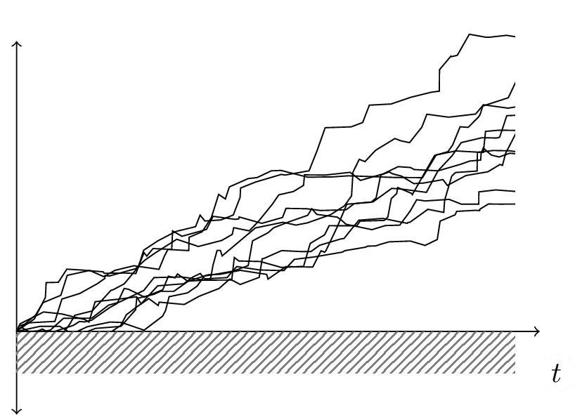
(a) Passive trend, there are more trajectories near 0.

(b) Driven trend, the trajectories have a drift towards an increased mean.

Of course, time runs on the vertical axis, but … what is in the horizontal one? Anything or, more precisely, anywhere the random diffusion takes place or the intended phenomenon “diffuses in”. In particular, the horizontal axis may quantify “biological complexity” whatever this may mean. The point Gould wants to clarify is in the difference between a fully random vs. a random and biased evolution. The biased right image does not apply to evolution: bacteria are still on Earth and very successfully. Any finalistic bias would instead separate the average random complexification from the left wall.

Note that, in both cases, complexity may locally decrease: tetrapodes may go back to the sea and lose their podia (the number of folding decreases, the overall body structure simplifies). Some cavern fishes may loose their eyes, in their new dark habitat; others, may lose their red blood cells (Ruud 1954). Thus, the local propagation of the original asymmetry may be biologically understood as follows: on average, variation by simplification leads towards a biological niches that has more chances to be already occupied. Thus, global complexity increases as a purely random effect of variability and on the grounds of local effects: the greater chances, for a “simpler” organism, to bump against an already occupied niche. Thus, more complex variants have just slightly more probabilities to survive and reproduce — but this slight difference is enough to produce, in the long run, very complex biological organisms. And, of course, variability and, thus, diversity are grounded on randomness, in biology. No need for finalism nor a priori “global aim” nor “design” at all, just a consequence of an original symmetry breaking in a random diffusion on a very peculiar phase space: biomass times complexity times time (see figure 3 for a complete diagram)^[8].

Similarly to embryogenesis, the complexification is a form of local reversal of entropy. The global entropy of the Universe increases (or does not decrease), but locally, by using energy of course, life inverses the entropic trend and creates organization of increasing complexity. Of course, embryogenesis is a more canalized process, while evolution seems to explore all “possible” paths, within the ecosystem-to-be. Most turn out to be incompatible with the environment, thus they are eliminated by selection. In embryogenesis increasing complexity seems to follow an expected path and it is partly so. But only in part as failures, in mammals say, reach $50\%$ or more: the constraints imposed, at least, by the inherited dna and zygote, limit the random exploration due to cell mitosis. Yet, their variability, joint to the many constraints added to development (first, a major one: dna), is an essential component of cell differentiation. Tissue differentiation is, for our point of view, a form of (strongly) regulated/canalized variability along cell reproduction.

Thus, by different but correlated effects, complexity as organization increases, on average, and reverts, locally, entropy. We called anti-entropy, Bailly and Longo ( 2009), this observable opposing entropy, both in evolution and embryogenesis; its peculiar nature is based on reproduction with random variation, submitted to constraints. As observed in the footnote above, anti-entropy differs from negentropy, which is just entropy with a negative sign, also because, when added to entropy, it never gives $0$, but it is realized in a very different singularity (different from $0$): extended criticality (Bailly and Longo 2011; Longo and Montévil 2011). In the next section, we will use this notion to provide a mathematical frame for a further insight by Gould.

3 (Anti-)Entropy in Evolution.

In yet another apparently naïve drawing, Gould proposes a further visualization of the increasing complexity of organisms along Evolution. It is just a qualitative image that the paleontologist draws on the grounds of his experience. It contains though a further remarkable idea: it suggests the “phase space” (the space of description) where one can analyze complexification. It is bio-mass density that diffuses over complexity, that is, figure 2 qualitatively describes the diffusion of the frequency of occurrences of individual organisms per unity of complexity.

This is just a mathematically naive, global drawing of the paleontologist on the basis of data. Yet, it poses major mathematical challenges. The diffusion, here, is not along a spatial dimension. Physical observables usually diffuse over space in time; or, within other physical matter (which also amounts to diffusing in space). Here, diffusion takes place over an abstract dimension, “complexity”. But what does biological complexity exactly mean? Hints are given in Gould (1997): the addition of a cellular nucleus (from bacteria to eukaryotes), the formation of metazoa, the increase in body size, the formation of fractal structures (usually — new — organs) and a few more…. In a sense, any added novelty provided by the random “bricolage” of Evolution and at least for some time compatible with the environment, contributes to complexity. Only a few organisms become more complex over time, but, by the original symmetry breaking mentioned above, this is enough to increase the global complexity. Of course, the figure above is highly unsatisfactory. It gives two slices over time where the second one is somewhat inconsistent: where are dinosaurs at present time? It is just a sketch, but an audacious one if analyzed closely. Mathematics may help us to consistently add the third missing dimension: time.

A simple form of diffusion equation of $q$ in time $t$ over space $x$ is:

$$\begin{array}{lll}\hfill \frac{\partial q}{\partial t}=D\frac{{\partial }^{2}q}{\partial x^2}+Q\left(t,x\right)& & \hfill \text{(1)}\end{array}$$

where $Q\left(t,x\right)$ is a source term describing the situation at the origin of the process. Yet, in our case, the diffusion of this strange quantity, $m$, a bio-mass density, takes place over an even more unusual “space”, biological complexity, whatever the latter may mean. In Bailly and Longo (2009), we dared to further specify Gould’s hints for biological complexity, as a quantity $K=\alpha K_c+\beta K_m+\gamma K_f$ where $\alpha$, $\beta$, and $\gamma$ are the respective “weights” of the different types of complexity within the total complexity. The details are in Bailly and Longo ( 2009), let’s just summarize the basic ideas. So, $K_c$ (“combinatorial” complexity) corresponds to the possible cellular combinatoric; $K_m$ (“morphological” complexity) is associated to the forms which arise (connexity and fractal structures); $K_f$ (“functional” complexity) is associated to the relational structures supporting biological functions (metabolic and neuronal relations). We will discuss this approach in section 4.

$K$ is a tentative quantification of complexity as anti-entropy, in particular in biological evolution: the increase of each of its components (more cellular differentiation, more or higher dimensional fractal structures, richer networks … yield a more “complex” individual). Of course, many more observables and parameters may be taken into account in order to evaluate the complexity of an organism: Bailly and Longo (2009) provides just a mathematical basis and a biological core for a preliminary analysis (an application to ontogenesis as an analysis of C. Elegans development is also presented). They suffice though for a qualitative (geometric) reconstruction of Gould’s curve, with a sound extension to the time dimension.

As mentioned above, anti-entropy opposes, locally, to entropy: it has the same dimension, yet it differs from negentropy, since it does not sum up to $0$, in presence of an equal quantity of entropy. It differs also from information theoretic frame, where negentropy has been largely used, as negentropy (= information) is independent from coding and Cartesian dimensions. This is crucial for Shannon as well as for Kolmogorof-Chaitin information theories. Anti-entropy, instead, as defined above, depends on foldings, singularities, fractality … it is a geometric notion, thus, by definition, it is sensitive to codings (and to dimension).

The next step is to adapt eq. 1 to these new dimensions. Just use Gould’s observables and parameters, $m$ and $K$, that we specified some more, and write:

$$\begin{array}{lll}\hfill \frac{\partial m}{\partial t}=D\frac{{\partial }^{2}m}{\partial K^2}+Q\left(t,K\right)& & \hfill \text{(2)}\end{array}$$

But what is here $Q\left(t,K\right)$, the source term? In order to instantiate $Q$ by a specific function, but also in order to see the biological system from a different perspective (and get to the equation also by an “operatorial approach”), we then gave a central role, as an observable, to the “global entropy production”.

Now, in physics, energy, $E$, is the “main” observable, since Galileo inertia, a principle of energy conservation, to Noether’s theorems and Schrödinger’s equation. Equilibria, geodetic principles etc directly or indirectly refer to energy and are understood in terms of symmetry principles (see Bailly and Longo (2011)). At least since Schrödinger and his equation, in (quantum) physics, one may view energy as an operator and time as a parameter^[9].

As hinted above, in biology, also constitutive processes, such as anti-entropy growth (the construction and reconstruction of organization), produce entropy, since they also produce some (new) disorder (recall: at least the proteome, after a mitosis, is non-uniformly and randomly distributed in the new cells). In these far form equilibrium, dissipative (possibly even non-stationary) processes, such as Evolution and ontogenesis, energy turns out to be just one (very important) observable, a parameter to be precise. One eats (and this is essential) and gets fatter: production and maintenance of organization requires energy, but it yields a different observable, one that has a different dimension, tentatively defined by $K$ above, as organization. Typically, in allometric equations, so relevant in biology, energy or mass appear as a parameter. Thus, in our approach, the key observable is organization that is formed or renewed (anti-entropy production).

Moreover, entropy, as associated to all irreversible processes, from energy flows to anti-entropy production, is the observable which summarizes all ongoing phenomena; by its irreversibility, it is strongly linked (conjugated) to time.

In summary, we proposed to change the conceptual frame and the conceptual priorities: we associated the global entropy production $\sigma$ to the differential operator given by time, $\partial ∕\partial t$ (Schrödinger does this for energy, which is conjugated to time, in quantum physics). Thus, our approach allows to consider biological time as an “operator”, both in this technical sense and in the global perspective of attributing to time a key constitutive role in biological phenomena, from evolution to ontogenesis. But how to express this global observable?

In a footnote to Schrödinger (1944), Schrödinger proposes to analyze his notion of negative entropy as a form of Gibbs free energy $G$. We applied this idea to our anti-entropy $S^{-}$, where $S^{-}=-kK$ ( $k$ is a positive dimensional constant and $K$ is the phenotypic complexity). Now, $G=H-TS$, where $T$ is temperature, $S$ is entropy and $H=U+PV$ is the system’s enthalpy ( $U$ is the internal energy, $P$ and $V$ are respectively pressure and volume). By definition, the metabolism $R$ has the physical dimension of a power and corresponds to the difference between the fluxes of generalized free energy $G$ through the surface $\Sigma$:

$$\begin{array}{lll}\hfill R=\sum \left[J_G\left(x\right)-J_G\left(x+dx\right)\right]=-\sum dx\left(Div{J}_G\right)& & \hfill \text{(3)}\end{array}$$

Locally the conservation (or balance) equation is expressed in the general form:

$$\begin{array}{lll}\hfill R=-Div{J}_G=\frac{dG}{dt}+T\sigma & & \hfill \text{(4)}\end{array}$$

where $\sigma$ represents the speed of global production of entropy, that is $\sigma$ is the entropy produced by all irreversible processes, including the production of biological organization or anti-entropy. Thus, the global balance of metabolism for the “system of life” (the biosphere) has the following form, where $S^{-}$ and $S^{+}$ are anti-entropy and entropy, respectively:

$$\begin{array}{lll}\hfill R=\frac{dH}{dt}-T\left.\frac{d{S}^{-}}{dt}+\frac{d{S}^{+}}{dt}\right)+T\sigma \simeq a\frac{dM}{dt}-T\left.\frac{d{S}^{-}}{dt}+\frac{d{S}^{+}}{dt}\right)+T\sigma & & \hfill \text{(5)}\end{array}$$

where $H\simeq aM$, for a mass $M$ and a coefficient $a$, which has the magnitude of a speed squared.

$T\sigma$ is a crucial quantity: it contains our $\sigma$, modulo the temperature $T$, since $R$ is a power. $T\sigma$ corresponds to the product of forces by fluxes (of matter, of energy — chemical energy, for instance — etc.). Now, a flux is proportional to a force, thus to a mass, and hence $T\sigma$ is proportional to a mass squared. It can then be written, up to a coefficient ${\zeta }_b$ and a constant term $T{\sigma }_0$ as:

$$\begin{array}{lll}\hfill T\sigma \approx {\zeta }_b{M}^2+T{\sigma }_0& & \hfill \text{(6)}\end{array}$$

${\zeta }_b$ is a constant that depends only on the global nature of the biological system under study and it is $0$ in absence of living matter.

Without entering into further details, by using as “state function” a bio-mass diffusion function over complexity $K$, that is the bio-mass density $m\left(t,K\right)$ in $t$ and $K$, the operatorial approach applied to equation 6 gave us the equation, with a linear source function ${\alpha }_{b}m$ :

$$\begin{array}{lll}\hfill \frac{\partial m}{\partial t}=D_b\frac{{\partial }^{2}m}{\partial K^2}+{\alpha }_{b}m& & \hfill \text{(7)}\end{array}$$

Its solution, bellow, yields the diagram in figure 3.

$$\begin{array}{lll}\hfill m\left(t,K\right)=\frac{A}{\sqrt{t}}exp\left(at\right)exp\left(-K^2∕4Dt\right)& & \hfill \text{(8)}\end{array}$$

In summary, by skipping all the technical details in Bailly and Longo (2009), we could derive, by mathematics and starting from Gould’s informal hints, a general understanding as well as the behavior of the “Evolution of complexity function” w. r. to time. And this fits data: at the beginning the linear source term gives an exponential growth of free bacteria. Then, they complexify and compete. Of course, this diagram, similarly to Gould’s, is a global one: it only gives a qualitative, geometric, understanding of the process. It is like looking at life on Earth from Sirius. Analogously to Gould’s diagram, the “punctuated equilibria”, say, and the major extinctions are not visible: the insight is from too far and too synthetic to appreciate them. It only theoretically justifies Gould’s proposal and soundly extends it to time dependence, by mathematically deriving it from general principles: the dynamics of a diffusion by random paths, with an asymmetric origin. Its source is given by an exponential growth. Life expansion is then bounded, canalized, selected in the interaction with the ever changing, co-constituted ecosystem. The core random complexification persists, while its “tail” exponentially decreases, see equation 8 and figure 3. In that tail, some neotenic big primates, with a huge neural network, turn out to be the random complexification of bacteria, a result of variability and of the immense massacres imposed by selection.

Another (important) analogy can be made with Schrödinger’s approach (his famous equation, not his book on life) and further justifies the reference to it for the analysis of this (rather ordinary) diffusion equation. Schrödinger dared to describe the deterministic evolution of the wave function in Quantum Mechanics as the dynamics of a law of probability (and this gives the intrinsic indetermination of the quantum system). We synthetically represented Biological Evolution as the dynamics of a potential of variability, under the left wall constraint. Again, this idea is essentially Gould’s idea in his 1996 book: he sees Evolution just as an asymmetric diffusion of random variability. We just made this point explicit and developed some computations as a consequences of the analogy with the determination in Quantum Mechanics and the operatorial approach of Schrödinger.

4 Anti-entropy as a measure of symmetry changes

In Longo and Montévil (2011), we proposed to understand biological phenomena, in comparison and contrast with physical theories, as a situation where the theoretical symmetries are “constantly” broken. We will now show that such considerations allows us to interpret anti-entropy, somewhat in the spirit of Boltzmann’s approach of physical entropy. In Bailly and Longo ( 2009), premises of these aspects are considered from a strictly combinatorial point of view, leading to a “constructive” definition of the three components of anti-entropy, we recalled in section 3. To show how symmetries come into play we will analyze now these components.

Combinatorial complexity, $K_c$:

For a total number of cells $N$ and for a number $n_j$ of cells of cell type $j$, the combinatorial complexity is defined as: $$\begin{array}{lll}\hfill K_c=log\left.\frac{N!}{\prod _j{n}_j!}\right)& & \hfill \text{(9)}\end{array}$$

A classical combinatorial point of view consists in saying that it is the number of ways to classify $N$ cells in $j$ categories each of sizes $n_j$. More precisely, we recognize, inside the logarithm, the cardinal, $N!$, of the symmetry group $S_N$, that is the group of transformations, called permutations, that exchange the labels of $N$ elements. Similarly, $n_j!$ is the number of permutations among $n_j$ units, which has the biological meaning of permutations of cells within a cell type: in other words, permuting cells within the same cell type is a combinatorial invariant of the complexity of an organism. Thus, the group of permutations leaving the cell types invariants is the group $G_{type}=\prod S_{n_j}$, that is the group obtained as direct product of the symmetries corresponding to permutations within each cell type. Formally, this group corresponds to the change of labels in each cell type, which can all be performed independently and conserve the classification by cell types. The cardinal of this group is ${\prod }_j{n}_j!$.

Then, the number of cell type configurations is the number of orbits generated by the right action of $G_{type}$ on $S_N$. In other words, a cell type configuration is first given by a permutation of $⟦1,N⟧$, which gives the random determination for $N$ cells. Moreover, these transformations must be computed modulo any transformation of $G_{type}$ that gives the same configuration (as we said, cells within each cell type are combinatorially equivalent — we will discuss below this hypothesis, in more biological terms). Lagrange theorem then gives the number of remaining transformations $N!∕{\prod }_j{n}_j!$, which is the number of possible configurations. Clearly, an organism with just one cell type (typically, a unicellular being) has combinatorial complexity $0$. As a result, this measure of combinatorial complexity depends on the total number $N$ of cells, but is actually a measure of the symmetry breaking induced by the differentiation in cell types.

Let’s compare the situation with Boltzmann approach of entropy. If one has a number of microscopic phase space states $\Omega$ having the same energy, the corresponding entropy is defined as $S=k_{b}log\left(\Omega \right)$. In the case of gases, one considers that the particles are indiscernible. This means that one does not count twice situations which differ only by permuting particles. In other words one formally understands the situation by saying that labels attached to particles are arbitrary. Thus, more soundly, $S$ is defined by $S=k_{b}log\left(\Omega \right)-k_{b}log\left(N!\right)>0$. This symmetry by permutation reduces the size of the microscopic possibility space, and, as a result, entropy.

In our approach, we have $K_c=log\left(N!\right)-{\sum }_{i}log\left(n_i!\right)$ which is greater than $0$, as soon as there is more than one cell type. Thus, the increase of the possibility space (the diversity or the differentiations) increases the complexity. More precisely, the complexity, as absolute value of anti-entropy, is decreased by the remaining symmetries, quantified by the term ${\sum }_{i}log\left(n_i!\right)$. We understand then that anti-entropy can be analyzed, at least in this case, as an account of how much biological symmetries are broken by the cascade of differentiations. Formally, we can sum the situation up by saying that the combinatorial complexity and its contribution to anti-entropy are based on a group of transformations, $S_N$, and a subgroup, $G_{type}$. The biologically relevant quantity is then the ratio of sizes of the groups $S_N$ and $G_{type}$.

Morphological complexity, $K_m$:

This complexity is associated to the geometrical description of biologically relevant shapes. It is computed in particular by counting the number of connex areas. Note that this number corresponds to space symmetry breakings for motions covering this space — or ergodic motions. Then, one has to consider the number of shape singularities, in the mathematical sense, where singularities are invariants by action of diffeomorphisms. The fractal-like structures are particularly relevant since they correspond to an exponential increase of the number of geometrical singularities with the range of scales involved. Thus, fractal-like structures lead to a linear growth of anti-entropy with the order of magnitudes where fractality is observed.

Functional complexity, $K_f$

(the last quantity proposed in Bailly and Longo (2009)): This quantity is given by the number of possible graphs of interaction. As a result, the corresponding component of anti-entropy is given by the choice of one graph structure (with distinguished nodes) among the possible graphs. This involves the selection of the structure of possible graphs and, correspondingly, which resulting graphs are considered equivalent. In terms of symmetries, we first have a symmetry among the possible graphs which is reduced to a smaller symmetry, by the equivalence relation. For example, in Bailly and Longo ( 2009), the case is considered where the number of edges is fixed, so the considered symmetry group is engendered by the transformations which combine the deletion of an edge and the creation of another one. The orbits preserve the total number of edges, so that the orbit of a graph with $⟨k⟩N$ edges are the graphs with this number of edges.

We understand then that anti-entropy, or at least its proposed decomposition in Bailly and Longo (2009), is strictly correlated to the amount of symmetry changes. We will now look more closely at the case of combinatorial complexity since it involves only the groups of permutations and their subgroups, but at the same time will also allow us to express a crucial conceptual and mathematical point.

We indeed encounter a paradox in the case of combinatorial complexity. On one side, we have an assumption that cells of the same cell type are symmetric (interchangeable). On the other, in section 1, we stressed that each cell division consists in a symmetry change. This apparent paradox depends on the scale we use to analyze the problem, as well as on the “plasticity” of the cells in a tissue or organ, as the possibility to be interchanged and/or to modify their individual organization. Typically, one can assume that liver cells function statistically (what matters is their average contribution to the function of the organ), while neurons may have strong specific activities, yet they may also deeply modify their structure (change number, forms and functionality of synaptic connections, for example). Thus, we will next consider the individual contribution of cells to the combinatorial complexity of an organism at different scales.

If we consider an organism with a large number of cells, $N$, and the proportion $q_j$ for cell type $j$ we get two different quantities for the combinatorial complexities, $K_{c1}$ and $K_{c2}$ :

$$\begin{array}{lllll}\hfill \frac{K_{c1}}{N}& =\frac{log\left(N!\right)}{N}\simeq log\left(N\right)& \hfill \frac{K_{c2}}{N}& =\frac{log\left.\frac{N!}{\prod _j\left(q_{j}N\right)!}\right)}{N}\simeq \sum _j{q}_{j}log\left(1∕q_j\right)& \hfill \text{(10)}\end{array}$$

We propose to understand the situation as follows. Basically, both levels of cellular individuation are valid; but they have to be arranged in the right order. Cellular differentiation is the first and main aspect of the ability of cells to individuate in a metazoan, so we can assume that the main determinant of combinatorial complexity is $K_{c2}$. It is only after this contribution that the further process of cellular individuation occurs. The latter leads to a mean contribution which is ${\sum }_j{a}_j\left.q_{j}log\left(q_{j}N\right)-1\right)$ per cell, where $a_j$ quantifies the ability of each cell type to change their organization. It seems reasonable to expect that the $a_j$ are high in the cases, for example, of neurons or of cells of the immune system. On the contrary, the $a_j$ should be especially low for red blood cells. The reason for this is not only their lack of dna, but also their relatively simple and homogeneous cytoplasmic organization. Similarly, liver cells may have statistically irrelevant changes in their individual structure.

Thus, the contribution of cell types to anti-entropy derives first from the formation of new cell types, while considering the ability of cells to reproduce, with changes, within a cell type as a further important (numerically dominant) aspect of their individuation process. Note that this analysis does not suppose that a cell type for a cell is irreversibly determined, but it means that the contribution of cell type changes to anti-entropy are understood as changes of $K_{c2}$.

We can then provide a refined version of $S_c^{-}$, where $a_{ct}$ is the “weight” accorded to the formation of different cell types:

$$\begin{array}{lll}\hfill \frac{S_c^{-}}{-N{k}_b}& =a_{ct}\sum _j{q}_{j}log\left(1∕q_j\right)+\sum _j{a}_j\left.q_{j}log\left(q_{j}N\right)-1\right)& \hfill \text{(11)}\\ \hfill & =\left.a_{ct}-⟨a_j⟩\right)log\left(1∕q_j\right)⟩+\left.⟨a_j⟩-a_j\right)log\left(1∕q_j\right)⟩+⟨a_j⟩log\left(N\right)& \hfill \text{(12)}\end{array}$$

where $⟨x⟩$ is the mean of $x$ among all cells (so that the contribution of each cell type is proportional to its proportion in the organism). Both equations 11 and 12 are biologically meaningful. The terms in equation 11 correspond, by order of appearance, to the contribution of the categorization by cell types and to the contribution of individuation among a cell type. In equation 12, we have obtained terms that can be assimilated to $K_{c1}$ (last term) and to $K_{c2}$ (first term), the latter being positive only if $a_{ct}-⟨a_j⟩>0$, meaning that the contribution associated to cell types is positive only if it is greater than the mean cellular individuation. This is logical since cell types make a positive contribution to the complexity only if the amount of cellular diversity they introduce is greater than the one that cellular individuation alone would introduce.

Last but not least, the second term has the sign of an anti-correlation between $a_j$ and $log\left(1∕q_j\right)$, meaning that this term is positive when there are many low complexity cell types^[10] and few high complexity cell types. More precisely, using the Cauchy-Schwartz equality case, we get that maximizing (and minimizing) this term (everything else being kept constant), leads to $⟨a_j⟩-a_j\propto log\left(1∕q_j\right)-⟨log\left(1∕q_j\right)⟩$. Then this optimization a priori leads to maximizing the variance of information (in informational terms), at constant entropy (=mean information).

Here, the issue derived from looking with an increasing finer resolution at the individuation potential. However, the reciprocal situation can also occur. Let’s consider the functional complexity, understood as the possibility of interactions between cells (the paradigmatic example is neurons). Then, by assuming that there are $N$ neurons with $⟨k⟩$ average number of synapses for each neuron (where $⟨k⟩$ is between 10³ and 10⁴ for humans), as presented in Bailly and Longo (2009), we get:

$$\begin{array}{lllll}\hfill N_G& =\left.\genfrac{}{}{0.0pt}{}{\left.\genfrac{}{}{0.0pt}{}{N}{2}\right)}{⟨k⟩N}\right)& \hfill \frac{K_{f1}}{N}& \simeq ⟨k⟩log\left(N\right)& \hfill \text{(13)}\end{array}$$

However, if we postulate that any graph of interaction is possible, then we get a total number of possible interactions which corresponds to a choice between interaction or no interaction for each entry of the interaction matrix ( $N^2$ cells). However, the latter is symmetric; and we do not count the self-interactions (because they correspond to the complexity of the cell) so we obtain $N\left(N-1\right)∕2$ binary choices, so $2^{n\left(n-1\right)∕2}$ possibilities: $K_{f2}∕N\simeq N∕2$.

There is two main lines of reasoning we can follow to understand the situation. The first is to look at the time structure of symmetry changes. Indeed, the symmetry changes occur as a temporal cascade. As a result, the temporal hierarchy of individuation is crucial. Here, we can refer to some phenomena concerning the graph of interaction of neurons. A crude description of the formation of neural networks is the following. First, a large number of “disordered” connections take place. Only after, the functional organization really increases by the decay of unused synapses (see for example Luo and O’Leary (2005). Then, the “bigger” symmetry group involved in the description is of the form $K_{f1}$, with $⟨k⟩$ mean number of connections; but then this symmetry group is reduced to obtain a smaller symmetry group with $⟨l⟩$ mean number of connections. This operation can be seen as a change of symmetry groups, from the transformations preserving the number of connections with $⟨k⟩N$ connections to those preserving $⟨l⟩N$ connections.

Of course there are many other possible components for a measure of biological complexity. This proposal, defined as anti-entropy, provides just a tentative backbone for transforming the informal notion of “biological organizational complexity” into a mathematical observable, that is into a real valued function defined over a biological phenomenon. It should be clear that, once enriched well beyond the definition and the further details given in Bailly and Longo ( 2009), this is a proper (and fundamental) biological observable. It radically differs from the rarely quantified, largely informal, always discrete (informally understood as a map from topologically trivial structures to integer numbers) notion of “information”, still dominating in molecular circles, see Longo et al. ( 2012) for a critique of this latter notion.

5 Theoretical consequences of this interpretation

In the section above, we have been focused on technical aspects of the “microscopic” definition of anti-entropy. Using this method, we have seen that anti-entropy can mainly be understood in terms of symmetry changes. We will now consider the theoretical meaning of this situation in a more general way. As we exposed in Longo and Montévil (2011), we propose to understand biological systems as characterized by a cascade of symmetry changes. Now, our understanding of a “biological trajectory”, a philogenetic and ontogenetic path, as a cascade of symmetry changes yields a proper form of randomness to be associated to the construction and maintenance of biological organization. This perspective is particularly relevant for us, since it links the two theoretical approaches of the living state of matter that our team has introduced: anti-entropy (Bailly and Longo 2009) and extended criticality (Bailly and Longo 2008; Longo and Montévil 2011).

More precisely, in phylogenesis, the randomness is associated to the “choice” of different organizational forms, which occurs even when the biological objects are confronted with remarkably similar physical environment and physiological constraints. For example, the lungs of birds and mammals have the same function in similar conditions; but they have phylogenetic histories which diverged long ago and, extremely different structures.

This example is particularly prone to lead to approximate common symmetries, since it relates to a vital function (respiration and therefore gas exchanges) shared by a wide class of organisms. It is noteworthy that numerous theoretical studies have analyzed lungs by optimality principles (Horsfield 1977; West, Brown, and Enquist 1999; Gheorghiu et al. 2005). However, the optimality principles differ in these studies (minimum entropy production, maximum energetic efficiency, maximum surface/volume ratio, …). Accordingly, even among mammals, structural variability remains high. For example, Nelson, West, and Goldberger ( 1990) describe the differences in the geometrical scaling properties of human lungs on one side, and of rats, dogs and hamsters lungs on the other side. Moreover, Mauroy et al. (2004) show that the criteria of energetic optimality and of robustness for the gas exchanges, with respect to geometric variations, are incompatible. More generally, optimization criteria are not particularly theoretically stable. In particular robustness is a relative notion: it depends on the property considered as well as on the transformations with respect to which we expect it to be robust (Lesne 2008).

Similarly, the theoretical symmetries constituted in ontogenesis are the result of the interactions with the environment and of the developmental trajectory already followed at a given time. In our perspective, this trajectory must then be understood as a history of symmetry changes. And, of course, the situation at a given moment does not “determine” the symmetry changes that the object will undergo. This is a crucial component of the randomness of the biological dynamics, as we consider that random events are associated to symmetry changes. These events are given by the interplay of the organism with its own physiology (and internal milieu) and with its environment, the latter being partially co-constituted by the theoretical symmetries of the organism, since the relevant aspects of the environment depend also on the organism.

In other terms, the conservation, in biology, is not associated to the biological proper observables, the phenotype, and the same (physical) interface (e.g. energy exchange) with the environment may yield very different phenotypes; thus, there is no need to preserve a specific phenotype. In short, the symmetry changes occurring in an organism can only be analyzed in terms of the previous theoretical symmetries (biology is, first, an historical science) and the differences of the possible changes can be associated to different forms of randomness.

In the cases of symmetry breakings, the symmetry change corresponds to the passage to a subgroup of the original symmetry group. As a result, the theoretical possibilities are predefinable (as the set of subgroups of the original group). This typically occurs in the case of physical phase transitions, and the result is then a randomness associated to the choice of how the symmetry gets broken. For example, if an organism has an approximate rotational symmetry, this symmetry can be broken in a subgroup, for example by providing a particular oriented direction. We then have a rotational symmetry along an axis. This can again be broken, for example into a discrete subgroup of order $5$ (starfish).

Another situation corresponds to the case where the symmetry changes are constituted on the basis of already determined theoretical symmetries (which can be altered in the process). This can be analyzed as the formation of additional observables which are attached to or the result of already existing ones. Then these symmetry changes are associated with already determined properties, but their specific form is nevertheless not predetermined. A typical example is the case of physically non-generic behaviours that can be found in the physical analysis of some biological situations, see Lesne and Victor (2006). From the point of view of the theoretical structure of determination, it is then a situation where there are predetermined attachment points, prone to lead the biological system to develop its further organization on them. The form of the biological response to these organizational opportunities of complexification is not, however, predetermined and then generates an original form of randomness. This theoretical account is close to the notion of next adjacent niche, proposed in Kauffman (2002); however, we emphasize, here, that the theoretical determination of these next organizational possibilities is only partially predetermined. For example imagine that a biological dynamic has approximately certain symmetries, which leads to a non-generic singular point; then it is possible (and maybe probable) that this point will be stabilized in evolution, in an unknown way.

The former case is constituted, in a sense, by a specific organizational opportunity. We can, however, consider cases where such opportunities are not theoretical predetermined. Now, the constitution of symmetry changes should be understood as even more random, and the associated predictability is extremely low. Gould’s most quoted example of “exaptation’, the formation of the bones of the internal hear from the double jaw of some tetrapods, some two hundred million years ago can fit in this category.

We have seen that the symmetry changes lead to a strong form of randomness. This randomness and its iterative accumulation are, however, the very fabric of biological organization. Therefore, we have a theoretical situation where order (biological organization) is a direct consequence of randomness. Its global analysis allowed us to give mathematical sense to Gould’s evolutionary complexification along evolution, as a consequence of the random paths of a asymmetric diffusion (sections 2 and 3). A finer (or local) analysis suggested a way to understand also ontogenetic changes in these terms, that is as a random dynamics of symmetry changes. This situation should be not confused with the cases of order by fluctuations or statistical stabilization (for example, by the central limit theorem). In our case, indeed, the order is not the result of a statistical regularization of random dynamics into a stable form, which would transform them into a deterministic frame. On the contrary, the random path of a cascade of symmetry changes yields the theoretical symmetries of the object (its specific phenotypes), which also determine its behaviour.

In this context, the irreversibility of these random processes is taken into account by entropy production. The latter, or more precisely a part of the latter, is then associated to the ability of biological objects to generate variability, thus adaptability. In ontogenesis, this point confirms our analysis of the contribution of anti-entropy regeneration to entropy production, in association with variability, including cellular differentiation. This situation is also consistent with our analysis of anti-entropy as a measure of symmetry changes. Notice that the symmetry changes, considered as relevant with respect to anti-entropy, may be taken into account, for example, in the coefficients corresponding to the individuation capacity of different cell types in our discussion above (see section 4).

References

1. Aoki, I. 1994. “Entropy production in human life span: A thermodynamical measure for aging.” AGE 17 (1): 29–31. issn: 0161-9152. doi: 10.1007/BF02435047. (Cited on page 6).
2. Bailly, F., and G. Longo. 2007. “Randomness and determinism in the interplay between the continuum and the discrete.” Mathematical Structures in Computer Science 17 (02): 289–305. doi:10.1017/S0960129507006007. (Cited on page 41).
3. _________. 2008. “Extended critical situations: the physical singularity of life phenomena.” Journal of Biological Systems 16 (2): 309. doi: 10.1142/S0218339008002514. (Cited on page 33).
4. _________. 2009. “Biological organization and anti-entropy.” Journal of Biological Systems 17 (1): 63–96. doi: 10.1142/S0218339009002715. (Cited on pages 4, 6 sqq., 12, 16 sq., 25, 28, 31 sq., 41).
5. _________. 2011. Mathematics and the natural sciences; The Physical Singularity of Life. London: Imperial College Press. (Cited on pages 13, 18).
6. d’Alessio, P. 2004. “Aging and the endothelium.” Experimental Gerontology 39 (2): 165–171. issn: 0531-5565. doi: 10.1016/j.exger.2003.10.025. (Cited on page 7).
7. Demetrius, L. 2004. “Caloric Restriction, Metabolic Rate, and Entropy.” The Journals of Gerontology Series A: Biological Sciences and Medical Sciences 59 (9): B902–B915. doi:10.1093/gerona/59.9.B902. (Cited on page 7).
8. Duffin, R.J., and C. Zener. 1969. “Geometric programming, chemical equilibrium, and the anti-entropy function.” Proceedings of the National Academy of Sciences 63 (3): 629. (Cited on page 41).
9. Gheorghiu, S., S. Kjelstrup, P. Pfeifer3, and M.-O. Coppens. 2005. “Is the Lung an Optimal Gas Exchanger?” In Fractals in Biology and Medicine, edited by Gabriele A. Losa, Danilo Merlini, Theo F. Nonnenmacher, and Ewald R. Weibel, 31–42. Mathematics and Biosciences in Interaction. Birkhäuser Basel. isbn: 978-3-7643-7412-9. doi: 10.1007/3-7643-7412-8˙3. (Cited on page 33).
10. Gould, S. J. 1989. Wonderful life: The Burgess Shale and the Nature of History. New York, USA: Norton. (Cited on pages 8 sq.).
11. _________. 1997. Full house: The spread of excellence from Plato to Darwin. Three Rivers Pr. (Cited on pages 8, 15 sq.).
12. Hardy, J. D. 1934. “The radiation of heat from the human body iii.” Journal of Clinical Investigation 13 (4): 615–620. doi: 10.1172/JCI100609. (Cited on page 5).
13. Hayflick, L. 2007. “Entropy Explains Aging, Genetic Determinism Explains Longevity, and Undefined Terminology Explains Misunderstanding Both.” PLoS Genet 3, no. 12 (December): e220. doi: 10.1371/journal.pgen.0030220. (Cited on pages 5 sq.).
14. Horsfield, K. 1977. “Morphology of branching trees related to entropy.” Respiration Physiology 29 (2): 179. doi: 10.1016/0034-5687(77)90090-1. (Cited on page 33).
15. Kauffman, S.A. 2002. Investigations. Oxford University Press, USA. (Cited on page 34).
16. Lambert, F.L. 2007. Entropy and the second law of thermodynamics. (Cited on page 5).
17. Lesne, A. 2008. “Robustness: Confronting lessons from physics and biology.” Biol Rev Camb Philos Soc 83 (4): 509–532. doi: 10.1111/j.1469-185X.2008.00052.x. (Cited on page 33).
18. Lesne, A., and J.-M. Victor. 2006. “Chromatin fiber functional organization: Some plausible models.” Eur Phys J E Soft Matter 19 (3): 279–290. doi: 10.1140/epje/i2005-10050-6. (Cited on page 34).
19. Lindner, A.B., R. Madden, A. Demarez, E.J. Stewart, and F. Taddei. 2008. “Asymmetric segregation of protein aggregates is associated with cellular aging and rejuvenation.” Proceedings of the National Academy of Sciences 105 (8): 3076–3081. doi:10.1073/pnas.0708931105. (Cited on page 6).
20. Longo, G. 2009. “Critique of Computational Reason in the Natural Sciences.” In Fundamental Concepts in Computer Science, edited by E. Gelenbe and J.-P. Kahane. Imperial College Press/World Scientific. (Cited on page 41).
21. Longo, G., P.-A. Miquel, C. Sonnenschein, and A. M. Soto. 2012. “Is information a proper observable for biological organization?” Progress in Biophysics and Molecular biology 109 (3): 108–114. issn: 0079-6107. doi: 10.1016/j.pbiomolbio.2012.06.004. (Cited on page 32).
22. Longo, G., and M. Montévil. 2011. “From physics to biology by extending criticality and symmetry breakings.” Progress in Biophysics and Molecular Biology 106 (2): 340–347. issn: 0079-6107. doi: 10.1016/j.pbiomolbio.2011.03.005. (Cited on pages 13, 25, 32 sq.).
23. _________. 2012. “Randomness Increases Order in Biological Evolution.” In Computation, Physics and Beyond, edited by M. Dinneen, B. Khoussainov, and A. Nies, 7160:289–308. Lecture Notes in Computer Science. Invited paper, Auckland, New Zealand, February 21-24, 2012. Springer Berlin / Heidelberg. isbn: 978-3-642-27653-8. doi: 10.1007/978-3-642-27654-5˙22. (Cited on page 41).
24. Luo, L., and D.M. O’Leary. 2005. “Axon retraction and degeneration in development and disease.” Annual Review of Neuroscience 28:127–156. doi: 10.1146/annurev.neuro.28.061604.135632. (Cited on page 32).
25. Marineo, G., and F. Marotta. 2005. “Biophysics of aging and therapeutic interventions by entropy-variation systems.” Biogerontology 6 (1): 77–79. issn: 1389-5729. doi: 10.1007/s10522-004-7387-6. (Cited on page 6).
26. Mauroy, B., M. Filoche, E.R. Weibel, and B. Sapoval. 2004. “An optimal bronchial tree may be dangerous.” Nature 427:633–636. doi: 10.1038/nature02287. (Cited on page 33).
27. McShea, D.W., and R.N. Brandon. 2010. Biology’s first law: the tendency for diversity and complexity to increase in evolutionary systems. University of Chicago Press. (Cited on page 41).
28. Nelson, T.R., B.J. West, and A.L. Goldberger. 1990. “The fractal lung: Universal and species-related scaling patterns.” Cellular and Molecular Life Sciences 46:251–254. doi:10.1007/BF01951755. (Cited on page 33).
29. Nyström, T. 2007. “A Bacterial Kind of Aging.” PLoS Genet 3 (12): e224. doi:10.1371/journal.pgen.0030224. (Cited on page 6).
30. Olshansky, S., and S. Rattan. 2005. “At the Heart of Aging: Is it Metabolic Rate or Stability?” Biogerontology 6:291–295. issn: 1389-5729. doi: 10.1007/s10522-005-2627-y. (Cited on page 7).
31. Pezard, J., L.and Martinerie, F.J. Varela, F. Bouchet, D. Guez, C. Derouesné, and B. Renault. 1998. “Entropy maps characterize drug effects on brain dynamics in Alzheimer’s disease.” Neuroscience Letters 253 (1): 5–8. issn: 0304-3940. doi:10.1016/S0304-3940(98)00603-X. (Cited on page 6).
32. Ruud, J.T. 1954. “Vertebrates without erythrocytes and blood pigment.” Nature 173 (4410): 848. (Cited on page 12).
33. Schrödinger, E. 1944. What Is Life? Cambridge U.P. (Cited on pages 5, 19).
34. Sohal, R.S., and R. Weindruch. 1996. “Oxidative stress, caloric restriction, and aging.” Science 273 (5271): 59–63. doi: 10.1126/science.273.5271.59. (Cited on page 7).
35. West, G.B., J.H. Brown, and B.J. Enquist. 1999. “The Fourth Dimension of Life: Fractal Geometry and Allometric Scaling of Organisms.” Science 284 (5420): 1677–1679. doi: 10.1126/science.284.5420.1677. (Cited on page 33).